An introduction to Finite Element Method

Krishna Kumar, kks32@cam.ac.uk
University of Cambridge

5R7 Lent 2018

Finite Element Analysis

FEA

Strong form

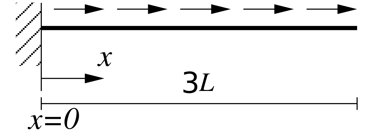
Strong form for a 1D bar

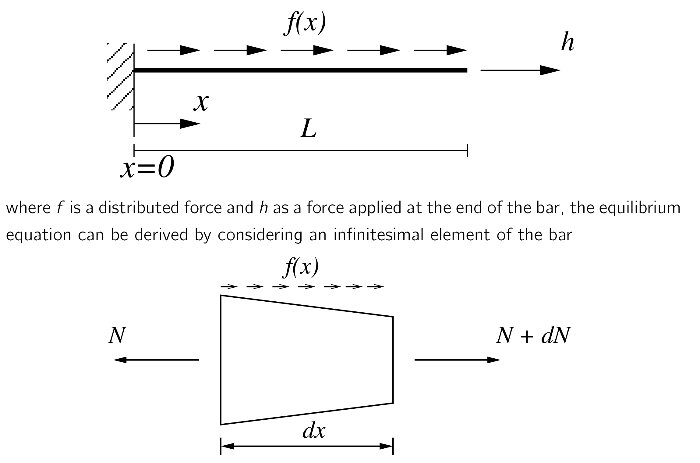
Strong form for a 1D bar

The forces $h$ acting at the ends of the bar are related to the normal force in the bar $N$ via $h = N n_x$, where $n_x$ is the ‘outward unit normal’ at the ends of the bar.

To satisfy equilibrium, forces acting on the bar must sum to zero.

$$0 = h(L) + h(0) + \int_{0}^{L}{f \mathrm{dx}} => N(L) - N(0) + \int_{0}^{L}{f \mathrm{dx}}$$ (since $h = Nn_x$) $$0 = \int_{0}^{L}{\frac{dN}{dx} \mathrm{dx}} + \int_{0}^{L}{f \mathrm{dx}}$$ All ‘smaller’ parts of the bar must also be in equilibrium, therefore we can remove the integrals, $-\frac{dN}{dx} = f$.

Strong form for a 1D bar

• Equilibrium equation: $ -\frac{dN}{dx} = f $
• Linear elasticity: $ N = A \sigma = EA \frac{du}{dx} = EA\epsilon $
• Inserting the constitutive model into the equilibrium equation: $$ -\frac{d}{dx}\left(EA\frac{du}{dx}\right) = f$$
• Boundary conditions:
  $u = 0$ at $x = 0$ (displacement or "Dirichlet" boundary condition)
  $EA\epsilon = h$ at $ x = L $ (force or "Neumann" boundary condition)

Converting Strong form to Weak form

The weak form is solved approximately using the finite element method

• Multiply the strong form equation by a weight function $v$ which is equal to zero where Dirichlet (displacement) boundary conditions are applied, but is otherwise arbitrary (must be sufficiently continous)
• Use integration by parts to `shift` derivatives to the weight fucntion
• Insert the Neumann (force) boundary conditions

Weak form for a 1D bar

• Multiply by weight function: $$ -\int_{0}^{L}v\frac{dN}{dx}dx = \int_{0}^{L}vf dx$$
• Integration by parts: $$ \int_{0}^{L}\frac{dv}{dx} N dx = \int_{0}^{L}vf dx + vN|_{x=0}^{x=L}$$
• Since $v(0) = 0$, inserting the constitutive relation and considering the force boundary at $x = L$: $$ \int_{0}^{L}\frac{dv}{dx} EA \frac{du}{dx} dx = \int_{0}^{L}vf dx + v(L)h$$

Finite Element formulation in 1D

• FE is a Galerkin method , which approximates a PDE by replacing the unknown function (the displacement $u$ in the case of the elastic bar) and the weight function $v$ by approximate fields ($u_h$ and $v_h$). Inserting these fields: $$ \int_{0}^{L}EA \frac{dv_h}{dx} \frac{du_h}{dx} dx = \int_{0}^{L}v_h f dx + v_h(L)h$$
• The approximate displacement field $u_h$ is defined using a set of basis functions $N_i(x)$ and values $a_i$ at a discrete number of points $x_i$ (known as nodes). For $n$ number of nodes, the approximate displacement field: $$ u_h(x) = \sum_{i}^{n} N_i (x) a_i$$
• In FE, the basis functions $N_i$ are "Shape functions" . The approximate strain field follows: $$ \epsilon_h = \frac{du_h}{dx} = \sum_{i}^{n}\frac{dN_i(x)}{dx} a_i$$

Basis functions

Finite Element formulation in 1D

• FE involves finding the coefficients of $a_i$, which gives approximate solution $u_h$ and $\epsilon_h$.
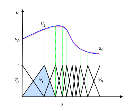
• The simplest FE basis function for 1D are hat-like continous piecewise linear polynomials. Each node $i$ has its own shape function and own dof. A shape function is equal to 1 at its own node and 0 at all others

  

Finite Element formulation in 1D

• Weakform: $$ \int_{0}^{L}EA \frac{dv_h}{dx} \frac{du_h}{dx} dx = \int_{0}^{L}v_h f dx + v_h(L)h$$
• Inserting expressions for $u_h$ and $v_h$: $$ \int_{0}^{L}EA \left(\sum_i^n\frac{dN_i}{dx}{a_i^*}\right)\left(\sum_j^n\frac{dN_j}{dx}{a_j}\right) = \int_{0}^{L}\left(\sum_i^nN_ia_i^*\right) f dx + \left(\sum_i^nN_i(L)a_i^*\right)h$$
• Since $a_i^*$ and $a_j$ are not functions of $x$: $$ \sum_i^n {a_i^*} \left(\sum_j^n {a_j} \int_{0}^{L}EA \frac{dN_i}{dx}\frac{dN_j}{dx}\right) = \sum_i^n a_i^*\int_{0}^{L}N_i f dx + \sum_i^nN_i(L)a_i^*h$$

Finite Element formulation in 1D

• Since $a_i^*$ is arbitrary for each $i$ we set $a_{k=i}^*=1$ and $a_{k \ne i}^*=1$. Then for each $i$ we have an equation with $n$ unknowns (the values of $a_j$): $$ i = 1: \sum_j^n {a_j} \int_{0}^{L}EA \frac{dN_1}{dx}\frac{dN_j}{dx} dx = \int_{0}^{L}N_1 f dx + N_i(L)h,$$ $$ i = 2: \sum_j^n {a_j} \int_{0}^{L}EA \frac{dN_2}{dx}\frac{dN_j}{dx} dx = \int_{0}^{L}N_2 f dx + N_i(L)h,$$ $$\dots$$ $$ i = n: \sum_j^n {a_j} \int_{0}^{L}EA \frac{dN_n}{dx}\frac{dN_j}{dx} dx = \int_{0}^{L}N_n f dx + N_i(L)h,$$
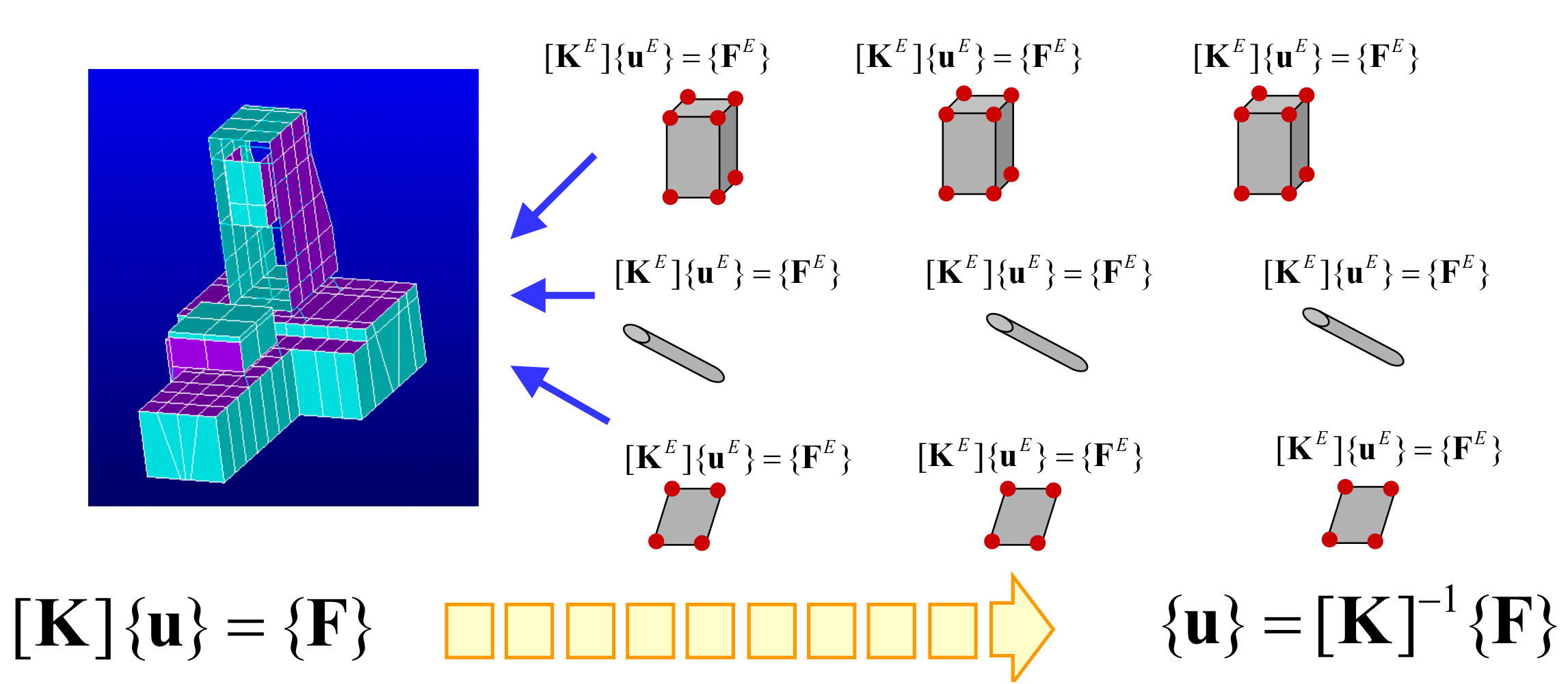
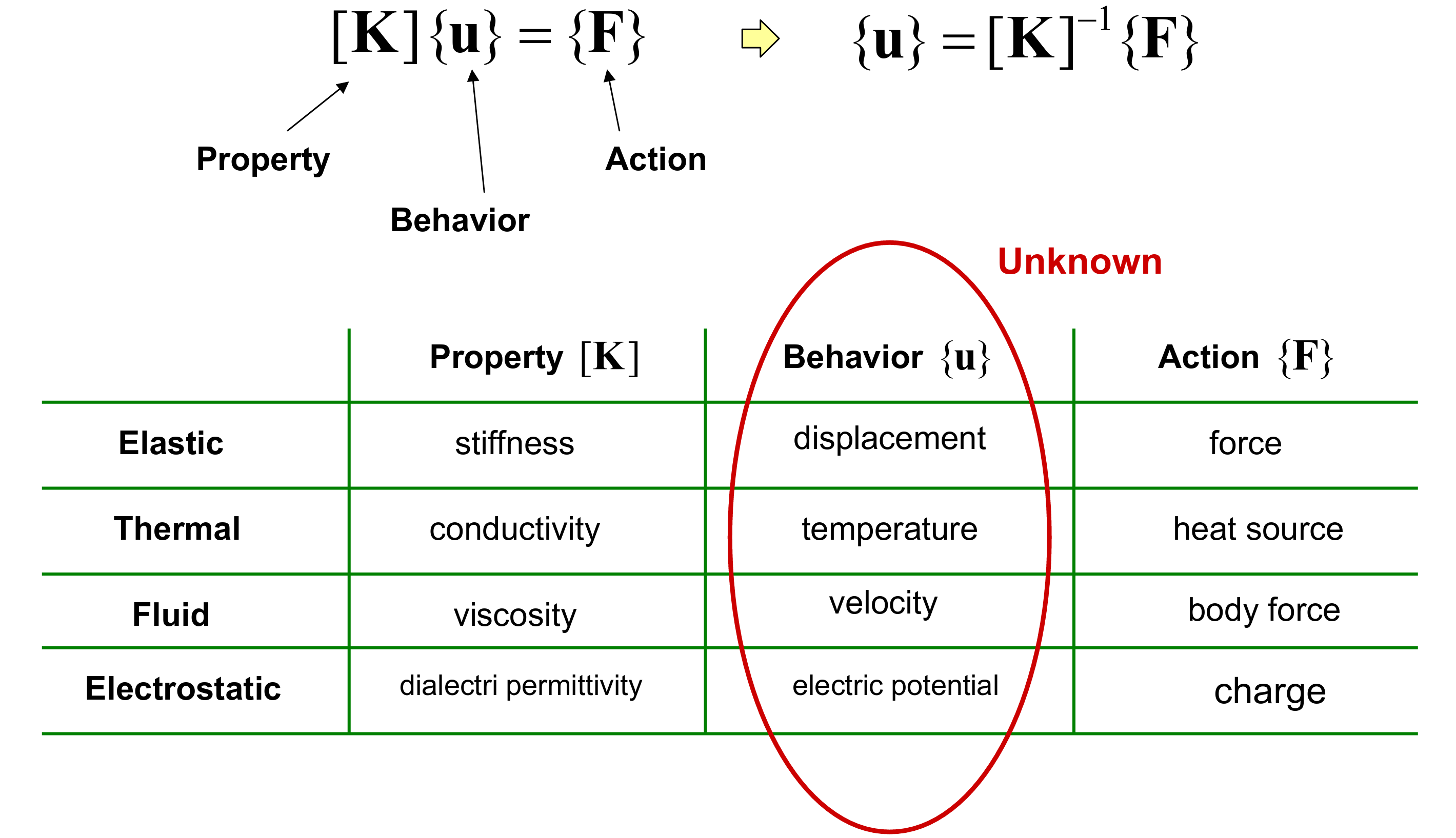
• A system of linear equationos is most conveniently expressed as a matrix: $$ \mathbf{K a} = \mathbf{b} $$
• Stiffness matrix: $K_{ij} = \int_{0}^{L}EA \frac{dN_i}{dx}\frac{dN_j}{dx} dx$
  right-hand side vector: $b_i = \int_{0}^{L}N_i f dx + N_i(L)h$.

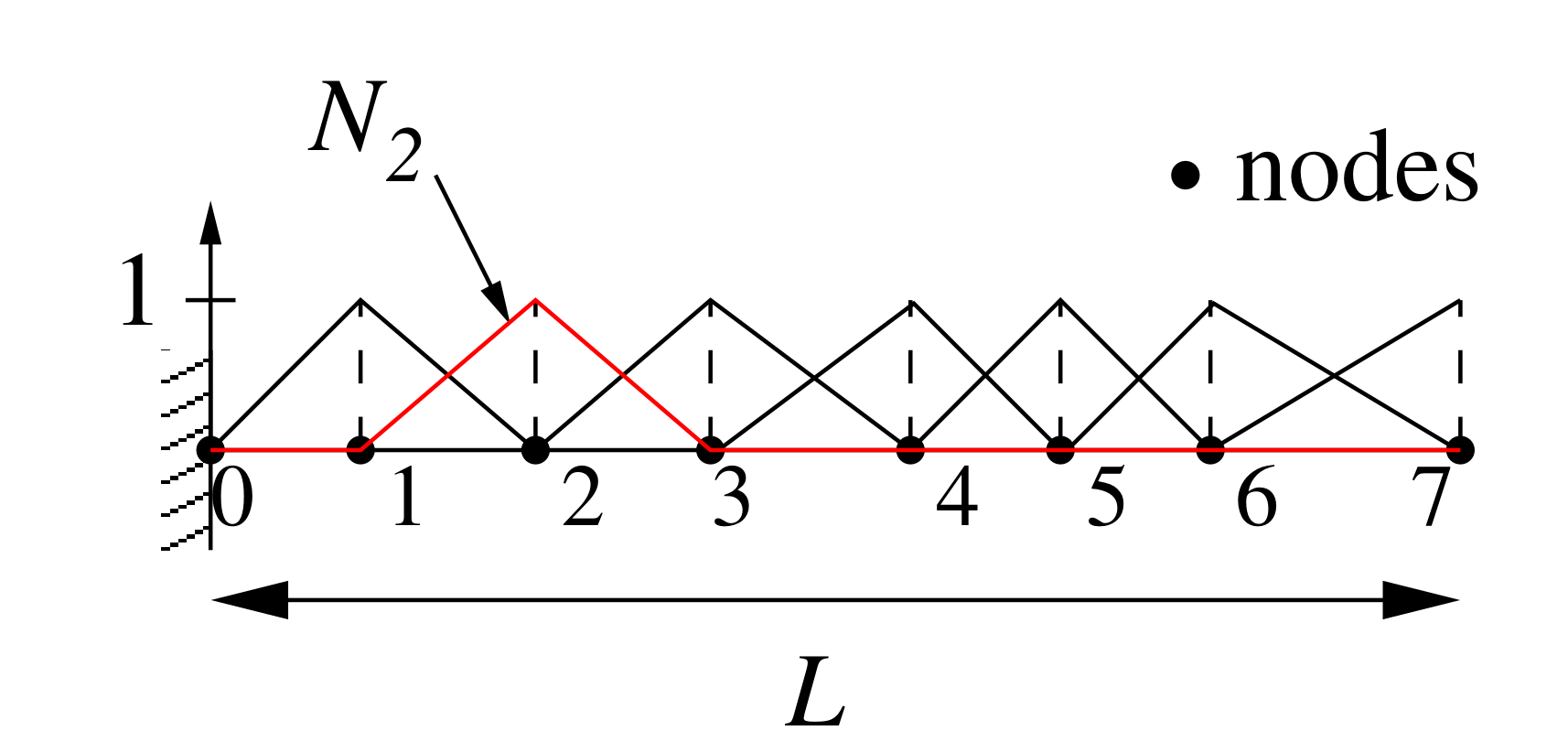
1D Shape functions

• Linear shape function between 2 nodes. Shape function is equal to 1 at its own node, and 0 at other nodes of the element:

  

• The displacement field: $u_h(x) = N_1(x) a_1 + N_2 (x) a_2 = (-\frac{x}{l} +1) a_1 + \frac{x}{l}a_2$
• The strain field: $\epsilon_h(x) = \frac{dN_1(x)}{dx} a_1 + \frac{dN_2 (x)}{dx} a_2 = -\frac{1}{l} a_1 + \frac{1}{l}a_2$
• In matrix format: $ u_h = \mathbf{Na_e} $ and $\epsilon_h = \mathbf{Ba_e}$.
• Shape function: $\mathbf{N} =\left[N_1(x) \quad N_2(x)\right]$ and derivatives: $\mathbf{B} = \left[ \frac{dN_1(x)}{dx} \quad \frac{dN_2(x)}{dx}\right]$

FE formulation: 1D element

• Stiffness matrix for 1D element: $K_{ij} = \int_{0}^{L} \frac{dN_i}{dx} EA \frac{dN_j}{dx} dx$
• FE matrix notation: $$K_{e} = \int_{0}^{L} \mathbf{B}^T EA \mathbf{B} dx$$
  $$K_{e} = \int_0^L \left[ \begin{matrix} \frac{dN_1}{dx} \\ \frac{dN_2}{dx} \end{matrix} \right] EA \left[ \begin{matrix} \frac{dN_1}{dx} & \frac{dN_2}{dx} \end{matrix} \right] dx$$
  $$K_{e} = \frac{EA}{l} \left[\begin{matrix} 1 & -1 \\ -1 & 1 \end{matrix} \right]$$

Finite Element Analysis of a Cantilever beam

Sleipner A offshore platform sprang leak

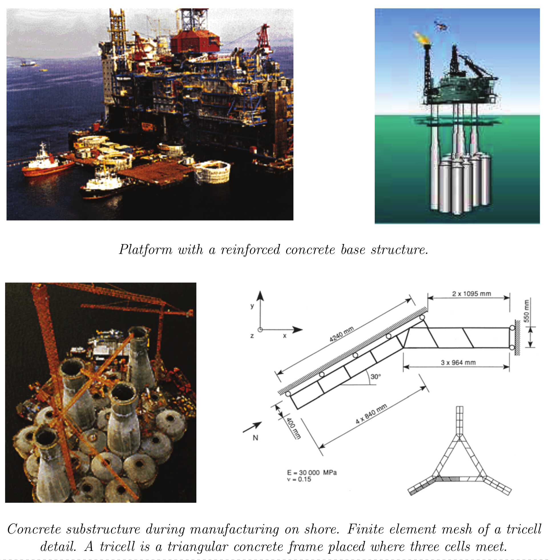
Using the finite element program NASTRAN, the shear stresses in the tricells were under- estimated by 47%. First, the chosen finite element mesh was exceedingly coarse so that the finite element shear stress was significantly too small.

Sleipner A offshore platform sprang leak

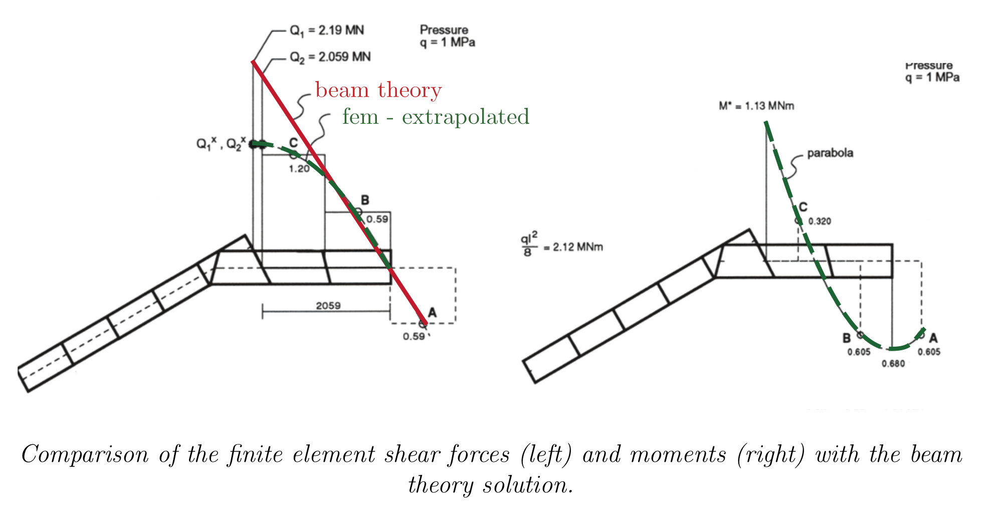
Second, the shear stresses at the boundary have been quadratically extrapolated using the shear forces at points A, B and C. We know however from beam theory that the shear force distribution is linear so that the shear force at the boundary is underestimated by ≈ 40%

Sleipner A offshore platform sprang leak

To make matters worse, the necessary reinforcement was automatically dimensioned based on the finite element results without any checking by an engineer.