Physics-Informed Neural Networks (PINNs)
Learning Objectives:
- Understand why standard neural networks fail for physics problems
- Learn how to incorporate physics into neural network training
- Master automatic differentiation for computing derivatives
- Compare data-driven vs physics-informed approaches
Exercise:
Solution:
Slides:
The Problem: A Damped Harmonic Oscillator
We begin with a concrete problem that everyone understands: a mass on a spring with damping. This is the perfect starting point because:
- Physical intuition: Everyone knows how springs work
- Mathematical tractability: We have an exact solution
- Clear demonstration: Shows why standard ML fails and PINNs succeed
The Physical System
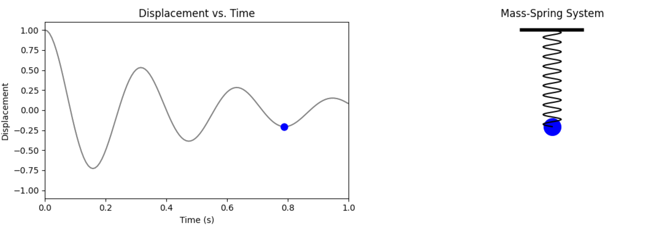
A mass $m$ attached to a spring (constant $k$) with damping (coefficient $c$). The displacement $u(t)$ from equilibrium satisfies:
$$m \frac{d^2 u}{dt^2} + c \frac{du}{dt} + ku = 0$$
Initial conditions: $u(0) = 1$, $\frac{du}{dt}(0) = 0$ (starts at rest, displaced)
Parameters: $m = 1$, $c = 4$, $k = 400$ (underdamped: $c^2 < 4mk$)
The Exact Solution
For underdamped motion ($\delta < \omega_0$ where $\delta = c/(2m)$ and $\omega_0 = \sqrt{k/m}$):
$$u(t) = e^{-\delta t}\left(\cos(\omega t) + \frac{\delta}{\omega}\sin(\omega t)\right)$$
where $\omega = \sqrt{\omega_0^2 - \delta^2}$ is the damped frequency.
This example is adapted from Ben Moseley's blog post.
import numpy as np
import matplotlib.pyplot as plt
import torch
import torch.nn as nn
import torch.optim as optim
from tqdm import tqdm
# Set random seeds for reproducibility
np.random.seed(42)
torch.manual_seed(42)
# Physical parameters
m = 1.0 # mass
c = 4.0 # damping coefficient
k = 400.0 # spring constant
# Derived parameters
delta = c / (2 * m) # damping ratio
omega_0 = np.sqrt(k / m) # natural frequency
omega = np.sqrt(omega_0**2 - delta**2) # damped frequency
print(f"Physical parameters:")
print(f" δ = {delta:.2f} (damping ratio)")
print(f" ω₀ = {omega_0:.2f} (natural frequency)")
print(f" ω = {omega:.2f} (damped frequency)")
print(f" Underdamped: {delta < omega_0}")
Physical parameters: δ = 2.00 (damping ratio) ω₀ = 20.00 (natural frequency) ω = 19.90 (damped frequency) Underdamped: True
import numpy as np
import matplotlib.pyplot as plt
from matplotlib.animation import FuncAnimation
from IPython.display import HTML
def oscillator(d, w0, x):
"""Analytical solution to the 1D underdamped harmonic oscillator problem."""
assert d < w0
w = np.sqrt(w0**2 - d**2)
phi = np.arctan(-d / w)
A = 1 / (2 * np.cos(phi))
cos = np.cos(phi + w * x)
exp = np.exp(-d * x)
y = exp * 2 * A * cos
return y
def create_spring_oscillator_animation_inline():
d = 2 # damping coefficient
w0 = 20 # natural frequency
# Animation variables
totalTime = 1.0 # Time domain [0, 1]
dt = 0.0075
t_array = np.arange(0, totalTime, dt)
y_array = oscillator(d, w0, t_array)
# Scaling factors
scale = 1.0
centerY = 0.0
# Compute y_min and y_max from the displacement data
y_min = np.min(y_array * scale + centerY)
y_max = np.max(y_array * scale + centerY)
# Create figure and axes
fig, (ax_trace, ax_spring) = plt.subplots(1, 2, figsize=(12, 4))
plt.tight_layout(pad=3.0)
# Plot the displacement curve on ax_trace
ax_trace.plot(t_array, y_array * scale + centerY, color='gray')
trace_point, = ax_trace.plot([], [], 'bo', markersize=8)
ax_trace.set_xlim(0, totalTime)
ax_trace.set_ylim(-1.1, 1.1)
ax_trace.set_xlabel('Time (s)')
ax_trace.set_ylabel('Displacement')
ax_trace.set_title('Displacement vs. Time')
# Set up the mass-spring system on ax_spring
ax_spring.set_xlim(-1, 1)
ax_spring.set_ylim(-1.1, 1.1)
ax_spring.axis('off')
ax_spring.set_title('Mass-Spring System')
# Draw the fixed block at equilibrium position (y=0)
ax_spring.plot([-0.2, 0.2], [1.0, 1.0], 'k-', linewidth=4)
# Initialize the mass and spring
mass, = ax_spring.plot([], [], 'bo', markersize=20)
spring_line, = ax_spring.plot([], [], 'k-', linewidth=1.5)
def get_spring(y_start, y_end, coils=10, points_per_coil=15):
length = y_end - y_start
t = np.linspace(0, 1, coils * points_per_coil)
x = 0.06 * np.sin(2 * np.pi * coils * t)
y = y_start + length * t
return x, y
def update(frame):
t = t_array[frame % len(t_array)]
y = oscillator(d, w0, t) * scale + centerY
# Update trace point
trace_point.set_data([t], [y])
# Update mass position
mass.set_data([0], [y])
# Update spring
x_spring, y_spring = get_spring(1.0, y) # Starting from y=1.0 (fixed point)
spring_line.set_data(x_spring, y_spring)
return trace_point, mass, spring_line
ani = FuncAnimation(fig, update, frames=len(t_array), interval=20, blit=True)
plt.close(fig)
return HTML(ani.to_jshtml())
# Call the function to display the animation
create_spring_oscillator_animation_inline()
Creating Sparse Training Data
In real applications, we don't have the complete solution. We only have sparse, potentially noisy measurements. Let's simulate this scenario:
# Generate sparse training data
n_data = 10 # Only 10 data points!
def exact_solution(t):
"""Analytical solution to the damped harmonic oscillator"""
return np.exp(-delta * t) * (np.cos(omega * t) + (delta/omega) * np.sin(omega * t))
# Get solution
t_data = np.linspace(0, 0.3607, n_data)
u_data = exact_solution(t_data)
# Exact solution
t_exact = np.linspace(0, 1, 500)
u_exact = exact_solution(t_exact)
# Add some noise to make it realistic
noise_level = 0.02
u_data_noisy = u_data + noise_level * np.random.normal(0, 1, len(u_data))
# Visualize the sparse data
plt.figure(figsize=(10, 6))
plt.plot(t_exact, u_exact, 'k--', linewidth=2, alpha=0.7, label='True solution')
plt.scatter(t_data, u_data_noisy, color='red', s=100, zorder=5, label=f'Training data ({n_data} points)')
plt.xlabel('Time t')
plt.ylabel('Displacement u(t)')
plt.title('The Challenge: Reconstruct the Full Solution from Sparse Data')
plt.legend()
plt.grid(True, alpha=0.3)
plt.show()
print(f"Training data: {n_data} points with noise level {noise_level}")
print("Challenge: Can a neural network reconstruct the full solution?")

Training data: 10 points with noise level 0.02 Challenge: Can a neural network reconstruct the full solution?
def exact_velocity(t):
"""
First derivative of the exact solution: du/dt
Given: u(t) = e^(-δt) * [cos(ωt) + (δ/ω)sin(ωt)]
Using product rule: d/dt[f(t)g(t)] = f'(t)g(t) + f(t)g'(t)
where f(t) = e^(-δt) and g(t) = cos(ωt) + (δ/ω)sin(ωt)
"""
exp_term = np.exp(-delta * t)
cos_term = np.cos(omega * t)
sin_term = np.sin(omega * t)
# Derivative of exponential term: d/dt[e^(-δt)] = -δe^(-δt)
d_exp_term = -delta * exp_term
# Derivative of trigonometric term: d/dt[cos(ωt) + (δ/ω)sin(ωt)]
d_trig_term = -omega * sin_term + (delta/omega) * omega * cos_term
d_trig_term = -omega * sin_term + delta * cos_term
# Apply product rule
velocity = d_exp_term * (cos_term + (delta/omega) * sin_term) + exp_term * d_trig_term
return velocity
def exact_acceleration(t):
"""
Second derivative of the exact solution: d²u/dt²
This can be computed by differentiating the velocity function,
or directly from the ODE: d²u/dt² = -(c/m)(du/dt) - (k/m)u
Using the ODE relation is more numerically stable:
m * d²u/dt² + c * du/dt + k * u = 0
Therefore: d²u/dt² = -(c/m) * du/dt - (k/m) * u
"""
u = exact_solution(t)
du_dt = exact_velocity(t)
# From the ODE: m * d²u/dt² = -c * du/dt - k * u
d2u_dt2 = -(c/m) * du_dt - (k/m) * u
return d2u_dt2
Stage 1: The Data-Only Approach (Why It Fails)
The Natural First Attempt: Train a neural network to fit the sparse data points.
Neural Network Architecture
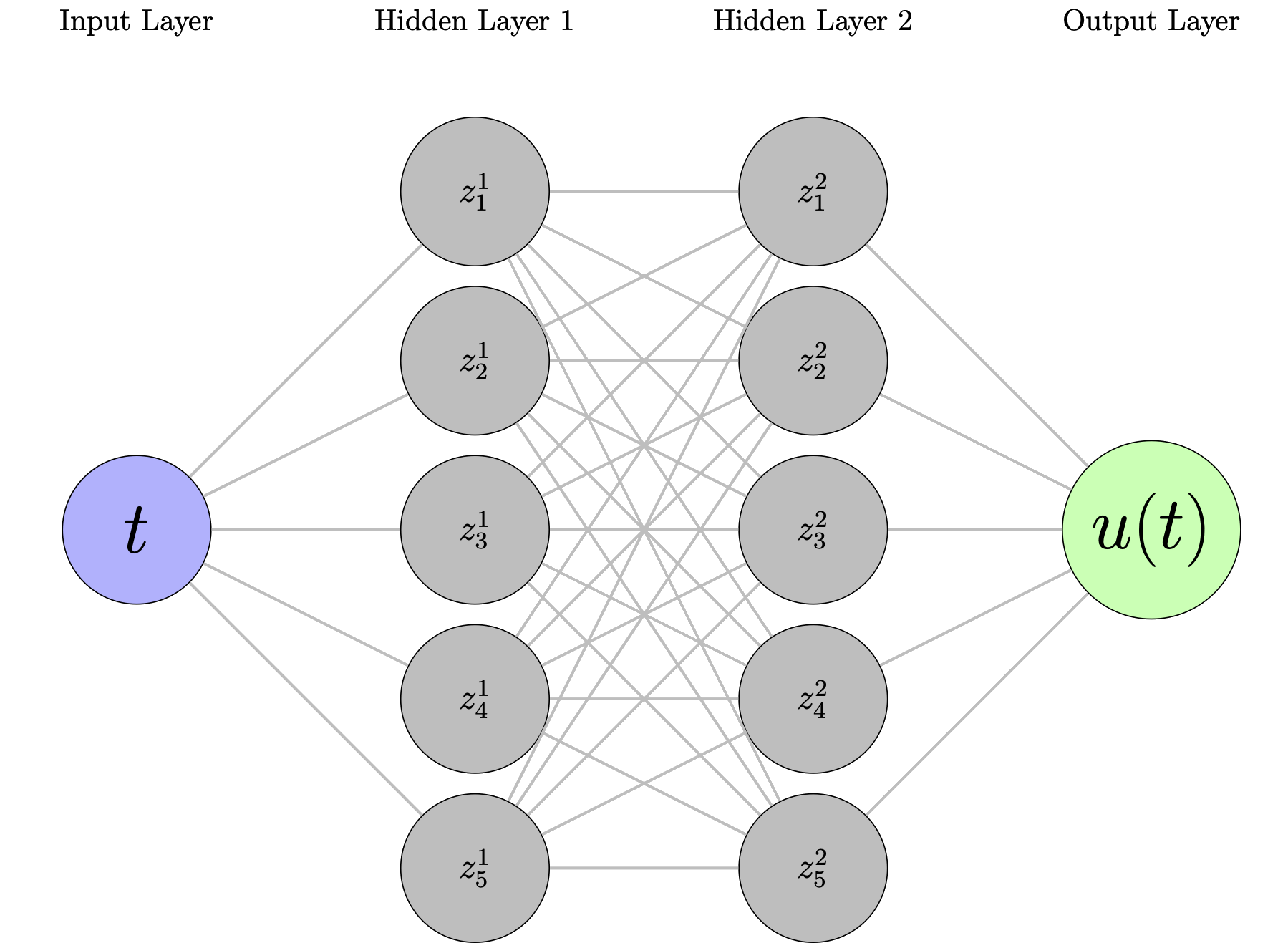
A simple feedforward network:
- Input: Time $t$
- Hidden layers: Dense layers with activation functions
- Output: Predicted displacement $\hat{u}_\theta(t)$
Loss function: Mean squared error between predictions and data $$\mathcal{L}_{\text{data}}(\theta) = \frac{1}{N} \sum_{i=1}^N |\hat{u}_\theta(t_i) - u_i|^2$$
Training: Standard gradient descent to minimize $\mathcal{L}_{\text{data}}$
Theoretical Foundation: Universal Approximation Theorem
Before we dive into implementation, we need to understand why neural networks can solve differential equations. The answer lies in the Universal Approximation Theorem and its extension to Sobolev spaces.
Classical Universal Approximation Theorem
As we learned in the MLP module, the classical UAT tells us that feedforward networks can approximate continuous functions:
Theorem (Cybenko, 1989): Let $\sigma$ be a continuous, non-constant, and bounded activation function. Then finite sums of the form: $$F(x) = \sum_{j=1}^N c_j \sigma(w_j \cdot x + b_j)$$ are dense in $C(K)$ for any compact set $K \subset \mathbb{R}^d$.
Translation: Given enough neurons, neural networks can approximate any continuous function arbitrarily well.
Extension to Sobolev Spaces: The Key for PDEs
But here's the critical insight: For differential equations, we don't just need to approximate functions—we need to approximate functions and their derivatives simultaneously.
This is where Sobolev spaces become essential.
Definition (Sobolev Space $H^k(\Omega)$): The space of functions whose weak derivatives up to order $k$ are square-integrable: $$H^k(\Omega) = \left\{ u : \Omega \to \mathbb{R} \,:\, \sum_{|\alpha| \leq k} \|D^\alpha u\|_{L^2(\Omega)}^2 < \infty \right\}$$
where $D^\alpha u$ denotes the weak derivative of multi-index $\alpha$ with $|\alpha| = \alpha_1 + \alpha_2 + \cdots + \alpha_d$.
Extended Universal Approximation Theorem: Neural networks with sufficiently smooth activation functions can approximate functions in Sobolev spaces $H^k(\Omega)$.
Mathematical Statement: Let $\sigma \in C^k(\mathbb{R})$ (i.e., $\sigma$ is $k$ times continuously differentiable). Then for any $u \in H^k(\Omega)$ and $\epsilon > 0$, there exists a neural network $\hat{u}_\theta$ such that: $$\|u - \hat{u}_\theta\|_{H^k} < \epsilon$$
where the Sobolev norm is: $$\|u\|_{H^k}^2 = \sum_{|\alpha| \leq k} \|D^\alpha u\|_{L^2}^2$$
Why This Matters for PINNs
Critical Connection: When we solve a differential equation of order $k$, we need:
- Function approximation: $\hat{u}_\theta(x) \approx u(x)$
- Derivative approximation: $\frac{\partial^j \hat{u}_\theta}{\partial x^j} \approx \frac{\partial^j u}{\partial x^j}$ for $j = 1, 2, \ldots, k$
The extended UAT guarantees this is possible provided:
- Activation function smoothness: $\sigma \in C^k$ (at least $k$ times differentiable)
- Sufficient network capacity: Enough neurons and layers
For our oscillator ODE: $m\frac{d^2u}{dt^2} + c\frac{du}{dt} + ku = 0$
- We need $k = 2$ (second-order equation)
- Activation function must be $C^2$ (twice differentiable)
- $\tanh$, $\sin$, Swish ✓ | ReLU ✗
The Magic: Automatic differentiation + UAT in Sobolev spaces = neural networks that can learn solutions to differential equations!"
class SimpleNN(nn.Module):
"""Standard feedforward neural network"""
def __init__(self, hidden_size=32, n_layers=3):
super().__init__()
layers = []
layers.append(nn.Linear(1, hidden_size)) # Input: time t
# Hidden layers
for _ in range(n_layers):
layers.append(nn.Tanh()) # Smooth activation (important!)
layers.append(nn.Linear(hidden_size, hidden_size))
layers.append(nn.Tanh())
layers.append(nn.Linear(hidden_size, 1)) # Output: displacement u
self.network = nn.Sequential(*layers)
def forward(self, t):
return self.network(t)
# Convert data to PyTorch tensors
t_data_tensor = torch.tensor(t_data.reshape(-1, 1), dtype=torch.float32)
u_data_tensor = torch.tensor(u_data_noisy.reshape(-1, 1), dtype=torch.float32)
t_test_tensor = torch.tensor(t_exact.reshape(-1, 1), dtype=torch.float32)
print("Data shapes:")
print(f" Training: {t_data_tensor.shape} -> {u_data_tensor.shape}")
print(f" Testing: {t_test_tensor.shape}")
Data shapes: Training: torch.Size([10, 1]) -> torch.Size([10, 1]) Testing: torch.Size([500, 1])
Training the Standard Neural Network
What we expect: The network should learn to pass through the data points.
What we hope: It will interpolate smoothly between points.
What actually happens: Let's find out!
def train_standard_nn(model, t_data, u_data, epochs=5000, lr=1e-3):
"""Train a standard neural network on data only"""
optimizer = optim.Adam(model.parameters(), lr=lr)
criterion = nn.MSELoss()
losses = []
# Training loop
pbar = tqdm(range(epochs), desc="Training Standard NN")
for epoch in pbar:
optimizer.zero_grad()
# Forward pass
u_pred = model(t_data)
# Data loss only
loss = criterion(u_pred, u_data)
# Backward pass
loss.backward()
optimizer.step()
losses.append(loss.item())
# Update progress bar with loss information every 100 epochs
if (epoch + 1) % 100 == 0:
pbar.set_postfix({'Loss': f'{loss.item():.6f}'})
return losses
# Create and train the standard neural network
standard_nn = SimpleNN()
losses_standard = train_standard_nn(standard_nn, t_data_tensor, u_data_tensor)
print(f"Final training loss: {losses_standard[-1]:.2e}")
Training Standard NN: 100%|██████████| 5000/5000 [00:01<00:00, 3569.44it/s, Loss=0.000001]
Final training loss: 1.00e-06
The Failure of the Data-Only Approach
Critical Question: How well does it predict the full solution?
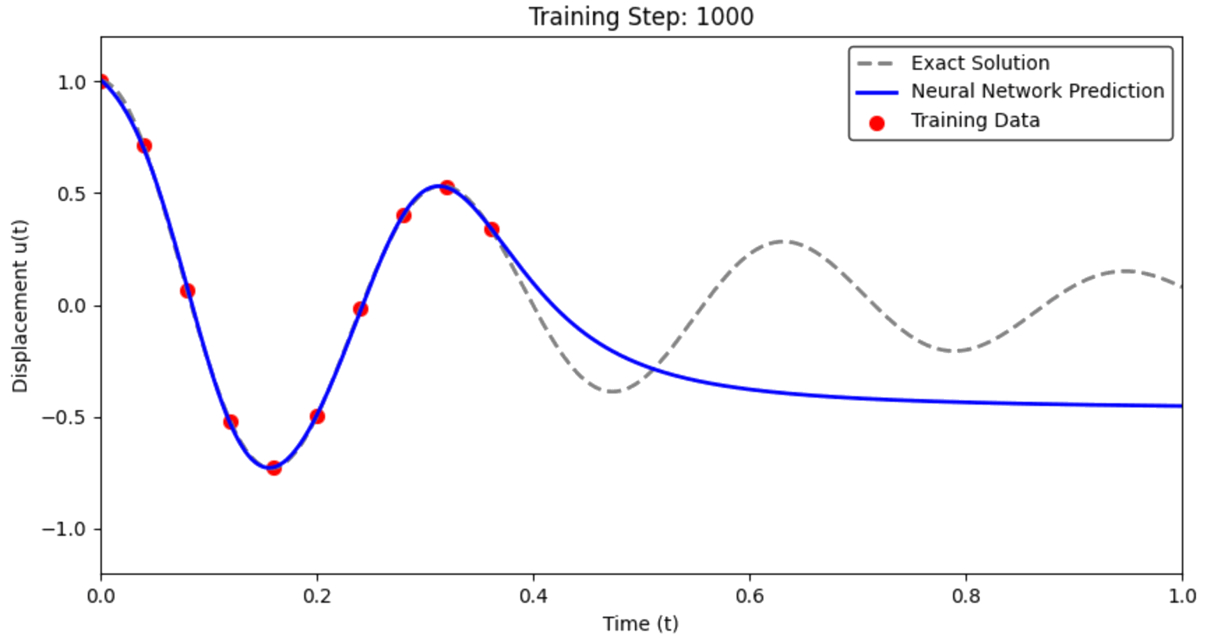
What we observe: The network fits the training points but fails catastrophically between them.
# Make predictions on the full time domain
with torch.no_grad():
u_pred_standard = standard_nn(t_test_tensor).numpy().flatten()
# Visualize the results
plt.figure(figsize=(12, 8))
# Plot 1: Full comparison
plt.subplot(2, 1, 1)
plt.plot(t_exact, u_exact, 'k-', linewidth=3, label='True solution', alpha=0.8)
plt.plot(t_exact, u_pred_standard, 'b--', linewidth=2, label='Standard NN prediction')
plt.scatter(t_data, u_data_noisy, color='red', s=80, zorder=5, label='Training data')
plt.xlabel('Time t')
plt.ylabel('Displacement u(t)')
plt.title('Standard Neural Network: Data-Only Training')
plt.legend()
plt.grid(True, alpha=0.3)
# Plot 2: Error analysis
plt.subplot(2, 1, 2)
error = np.abs(u_pred_standard - u_exact)
plt.plot(t_exact, error, 'r-', linewidth=2, label='Absolute error')
plt.scatter(t_data, np.zeros_like(t_data), color='red', s=80, zorder=5,
label='Training data locations')
plt.xlabel('Time t')
plt.ylabel('|Error|')
plt.title('Prediction Error vs Time')
plt.legend()
plt.grid(True, alpha=0.3)
plt.yscale('log')
plt.tight_layout()
plt.show()
# Compute metrics
mse = np.mean((u_pred_standard - u_exact)**2)
max_error = np.max(np.abs(u_pred_standard - u_exact))
print(f" Standard NN Performance:")
print(f" MSE: {mse:.6f}")
print(f" Max Error: {max_error:.6f}")

Standard NN Performance: MSE: 0.193027 Max Error: 0.799645
Stage 2: Enter Physics-Informed Neural Networks
The Key Insight: Instead of just fitting data, enforce the differential equation!
The PINN Architecture
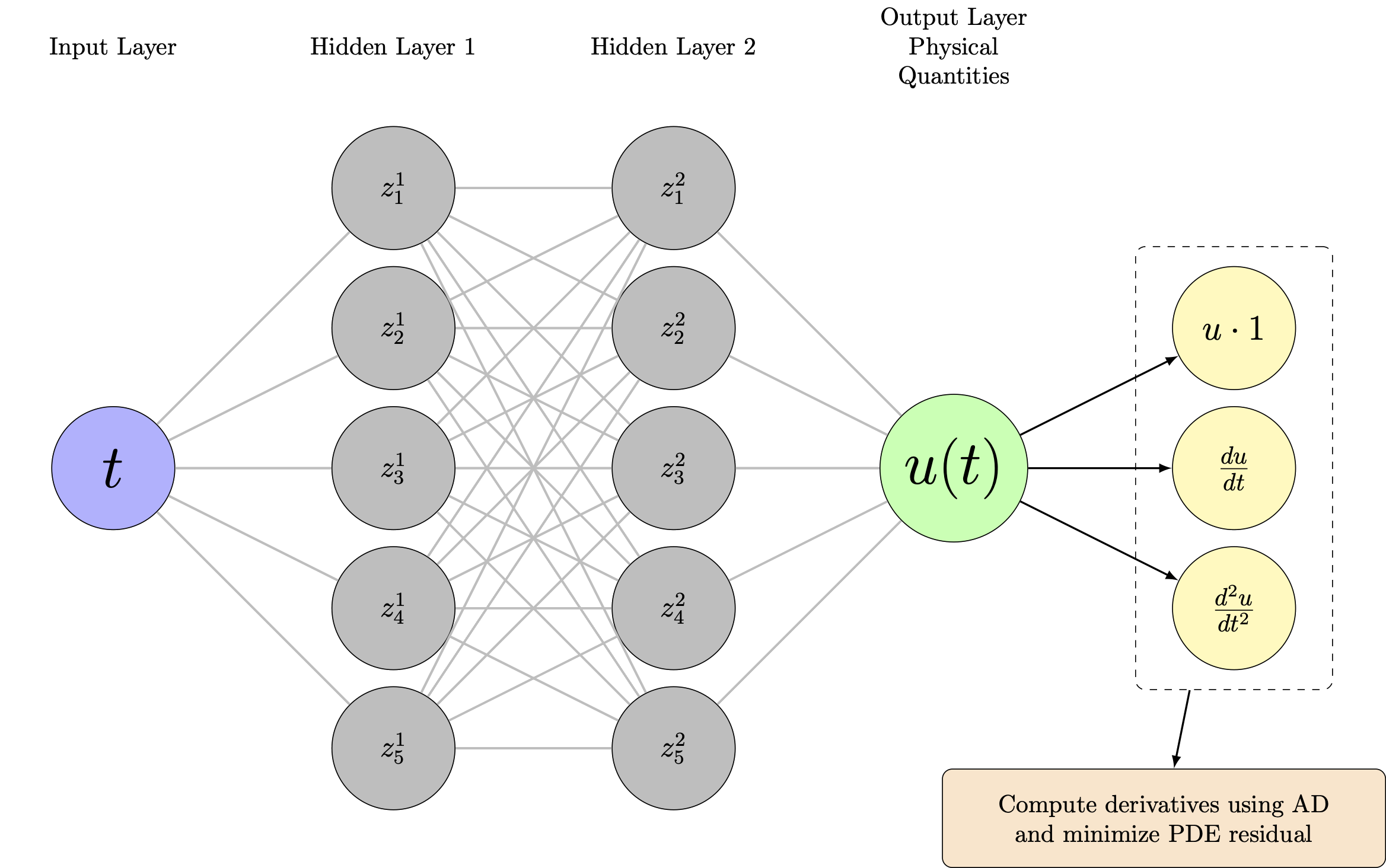
Same network, different loss function:
- Network still predicts $\hat{u}_\theta(t)$
- But now we compute derivatives via automatic differentiation
- Physics residual: $\mathcal{R}_\theta(t) = m\frac{d^2\hat{u}_\theta}{dt^2} + c\frac{d\hat{u}_\theta}{dt} + k\hat{u}_\theta$
The Physics Residual
Mathematical Foundation: If $\hat{u}_\theta(t)$ is the exact solution, then: $$m\frac{d^2\hat{u}_\theta}{dt^2} + c\frac{d\hat{u}_\theta}{dt} + k\hat{u}_\theta = 0$$
PINN Strategy: Make this residual as small as possible everywhere in the domain.
Collocation Points: We evaluate the residual at many points {t_j} throughout $[0,1]$, not just at data points.
The Complete PINN Loss Function
$$\mathcal{L}_{\text{total}}(\theta) = \mathcal{L}_{\text{data}}(\theta) + \lambda \mathcal{L}_{\text{physics}}(\theta)$$
where:
Data Loss: $\mathcal{L}_{\text{data}}(\theta) = \frac{1}{N_{\text{data}}} \sum_{i=1}^{N_{\text{data}}} |\hat{u}_\theta(t_i) - u_i|^2$
Physics Loss: $\mathcal{L}_{\text{physics}}(\theta) = \frac{1}{N_{\text{colloc}}} \sum_{j=1}^{N_{\text{colloc}}} |\mathcal{R}_\theta(t_j)|^2$
Balance Parameter: $\lambda$ controls data vs physics trade-off
Automatic Differentiation: The Secret Weapon
Critical Question: How do we compute $\frac{d\hat{u}_\theta}{dt}$ and $\frac{d^2\hat{u}_\theta}{dt^2}$?
Answer: Automatic differentiation (AD) gives us exact derivatives!
- No finite differences
- No numerical errors
- Computed via chain rule through the computational graph
- Available in PyTorch, TensorFlow, JAX
Demonstration: Automatic Differentiation in Action
Let's see how automatic differentiation works in PyTorch:
def compute_derivatives_demo():
"""Demonstrate automatic differentiation"""
# Create a simple test case: u(t) = sin(t)
t = torch.tensor([0.5], requires_grad=True) # Enable gradient computation
u = torch.sin(t) # u = sin(t)
print("Function: u(t) = sin(t)")
print(f"At t = {t.item():.2f}:")
print(f" u = {u.item():.6f}")
# First derivative: du/dt
du_dt = torch.autograd.grad(u, t, create_graph=True)[0]
print(f" du/dt = {du_dt.item():.6f} (exact: cos({t.item():.2f}) = {np.cos(t.item()):.6f})")
# Second derivative: d²u/dt²
d2u_dt2 = torch.autograd.grad(du_dt, t, create_graph=True)[0]
print(f" d²u/dt² = {d2u_dt2.item():.6f} (exact: -sin({t.item():.2f}) = {-np.sin(t.item()):.6f})")
print("✅ Automatic differentiation gives exact derivatives!")
compute_derivatives_demo()
Function: u(t) = sin(t) At t = 0.50: u = 0.479426 du/dt = 0.877583 (exact: cos(0.50) = 0.877583) d²u/dt² = -0.479426 (exact: -sin(0.50) = -0.479426) ✅ Automatic differentiation gives exact derivatives!
def physics_loss(model, t_colloc, m, c, k):
"""
Compute the physics loss for the damped harmonic oscillator
ODE: m * d²u/dt² + c * du/dt + k * u = 0
"""
# Ensure gradients are enabled for input
t_colloc = t_colloc.clone().detach().requires_grad_(True)
# Forward pass: compute u(t)
u = model(t_colloc)
# First derivative: du/dt
du_dt = torch.autograd.grad(
outputs=u,
inputs=t_colloc,
grad_outputs=torch.ones_like(u),
create_graph=True, # Allow higher-order derivatives
retain_graph=True
)[0]
# Second derivative: d²u/dt²
d2u_dt2 = torch.autograd.grad(
outputs=du_dt,
inputs=t_colloc,
grad_outputs=torch.ones_like(du_dt),
create_graph=True,
retain_graph=True
)[0]
# Physics residual: R = m * d²u/dt² + c * du/dt + k * u
residual = m * d2u_dt2 + c * du_dt + k * u
# Mean squared residual
physics_loss = torch.mean(residual**2)
return physics_loss
# Test the physics loss function
test_model = SimpleNN()
t_test_colloc = torch.linspace(0, 1, 50).reshape(-1, 1)
test_loss = physics_loss(test_model, t_test_colloc, m, c, k)
print(f"Physics loss (untrained model): {test_loss.item():.6f}")
print("This is large since the model hasn't learned the physics yet!")
Physics loss (untrained model): 202.440353 This is large since the model hasn't learned the physics yet!
Step 2: Complete PINN Training Loop
Key Components:
- Data loss: Fit the sparse measurements
- Physics loss: Satisfy the differential equation
- Collocation points: Where we enforce physics (not necessarily data points)
- Balance parameter $\lambda$: Controls the trade-off
def train_pinn(model, t_data, u_data, t_colloc, m, c, k,
epochs=10000, lr=1e-3, lambda_physics=1e-4):
"""
Train a Physics-Informed Neural Network
Args:
model: Neural network
t_data, u_data: Training data points
t_colloc: Collocation points for physics
m, c, k: Physical parameters
lambda_physics: Balance parameter between data and physics
"""
optimizer = optim.Adam(model.parameters(), lr=lr)
criterion = nn.MSELoss()
# Storage for loss history
data_losses = []
physics_losses = []
total_losses = []
print(f"Training PINN with λ = {lambda_physics}")
print(f"Data points: {len(t_data)}, Collocation points: {len(t_colloc)}")
pbar = tqdm(range(epochs), desc="Training PINN")
for epoch in pbar:
optimizer.zero_grad()
# Data loss: how well do we fit the measurements?
u_pred_data = model(t_data)
loss_data = criterion(u_pred_data, u_data)
# Physics loss: how well do we satisfy the ODE?
loss_physics = physics_loss(model, t_colloc, m, c, k)
# Total loss: balance data fitting and physics
total_loss = loss_data + lambda_physics * loss_physics
# Backpropagation
total_loss.backward()
optimizer.step()
# Store losses
data_losses.append(loss_data.item())
physics_losses.append(loss_physics.item())
total_losses.append(total_loss.item())
if (epoch + 1) % 2000 == 0:
pbar.set_postfix({'Loss': f'{loss_data.item():.6f}',
'Physics': f'{loss_physics.item():.6f}',
'Total': f'{total_loss.item():.6f}'})
return data_losses, physics_losses, total_losses
# Setup for PINN training
n_colloc = 200 # Number of collocation points
t_colloc = torch.linspace(0, 1, n_colloc).reshape(-1, 1)
lambda_physics = 1e-4 # Balance parameter
print(f"Collocation points: uniformly distributed in [0, 1]")
print(f"Physics weight λ = {lambda_physics} (typically much smaller than 1)")
# Visualize training setup
plt.figure(figsize=(10, 4))
plt.scatter(t_data, u_data_noisy, color='red', s=100, zorder=5, label='Data points (fit these)')
plt.scatter(t_colloc.numpy().flatten()[::10], np.zeros(len(t_colloc[::10])),
color='green', marker='^', s=60, alpha=0.7, label='Collocation points (enforce physics)')
plt.plot(t_exact, u_exact, 'k--', alpha=0.7, label='True solution')
plt.xlabel('Time t')
plt.ylabel('Displacement')
plt.title('PINN Training Setup: Data Points vs Collocation Points')
plt.legend()
plt.grid(True, alpha=0.3)
plt.show()
Collocation points: uniformly distributed in [0, 1] Physics weight λ = 0.0001 (typically much smaller than 1)

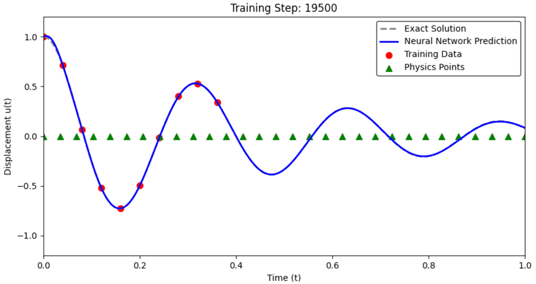
Step 3: Train the PINN
The moment of truth! Let's train the PINN and see if it can learn both the data and the physics:
# Create a fresh PINN model
pinn_model = SimpleNN()
# Train the PINN
data_losses, physics_losses, total_losses = train_pinn(
pinn_model, t_data_tensor, u_data_tensor, t_colloc, m, c, k, epochs=20000
)
# Make predictions
with torch.no_grad():
u_pred_pinn = pinn_model(t_test_tensor).numpy().flatten()
print(f"PINN Training Complete!")
print(f"Final data loss: {data_losses[-1]:.6f}")
print(f"Final physics loss: {physics_losses[-1]:.6f}")
Training PINN with λ = 0.0001 Data points: 10, Collocation points: 200
Training PINN: 100%|██████████| 20000/20000 [00:25<00:00, 799.02it/s, Loss=0.000249, Physics=1.498582, Total=0.000398]
PINN Training Complete! Final data loss: 0.000249 Final physics loss: 1.498582
# Compare Standard NN vs PINN
fig, axes = plt.subplots(2, 2, figsize=(15, 10))
# Plot 1: Solutions comparison
ax = axes[0, 0]
ax.plot(t_exact, u_exact, 'k-', linewidth=3, label='True solution', alpha=0.8)
ax.plot(t_exact, u_pred_standard, 'b--', linewidth=2, label='Standard NN', alpha=0.8)
ax.plot(t_exact, u_pred_pinn, 'r-', linewidth=2, label='PINN', alpha=0.8)
ax.scatter(t_data, u_data_noisy, color='red', s=80, zorder=5, label='Training data')
ax.set_xlabel('Time t')
ax.set_ylabel('Displacement u(t)')
ax.set_title('Solution Comparison')
ax.legend()
ax.grid(True, alpha=0.3)
# Plot 2: Error comparison
ax = axes[0, 1]
error_standard = np.abs(u_pred_standard - u_exact)
error_pinn = np.abs(u_pred_pinn - u_exact)
ax.plot(t_exact, error_standard, 'b-', linewidth=2, label='Standard NN error')
ax.plot(t_exact, error_pinn, 'r-', linewidth=2, label='PINN error')
ax.set_xlabel('Time t')
ax.set_ylabel('Absolute Error')
ax.set_title('Error Comparison')
ax.set_yscale('log')
ax.legend()
ax.grid(True, alpha=0.3)
# Plot 3: Loss evolution for Standard NN
ax = axes[1, 0]
ax.plot(losses_standard, 'b-', linewidth=2, label='Data loss only')
ax.set_xlabel('Epoch')
ax.set_ylabel('Loss')
ax.set_title('Standard NN Training')
ax.set_yscale('log')
ax.legend()
ax.grid(True, alpha=0.3)
# Plot 4: Loss evolution for PINN
ax = axes[1, 1]
ax.plot(data_losses, 'b-', linewidth=2, label='Data loss', alpha=0.8)
ax.plot(physics_losses, 'g-', linewidth=2, label='Physics loss', alpha=0.8)
ax.plot(total_losses, 'r-', linewidth=2, label='Total loss', alpha=0.8)
ax.set_xlabel('Epoch')
ax.set_ylabel('Loss')
ax.set_title('PINN Training (Multiple Loss Components)')
ax.set_yscale('log')
ax.legend()
ax.grid(True, alpha=0.3)
plt.tight_layout()
plt.show()
# Quantitative comparison
mse_standard = np.mean((u_pred_standard - u_exact)**2)
mse_pinn = np.mean((u_pred_pinn - u_exact)**2)
max_error_standard = np.max(np.abs(u_pred_standard - u_exact))
max_error_pinn = np.max(np.abs(u_pred_pinn - u_exact))
print("📊 QUANTITATIVE COMPARISON")
print("="*50)
print(f"{'Metric':<20} {'Standard NN':<15} {'PINN':<15} {'Improvement':<15}")
print("-"*65)
print(f"{'MSE':<20} {mse_standard:<15.6f} {mse_pinn:<15.6f} {mse_standard/mse_pinn:<15.1f}x")
print(f"{'Max Error':<20} {max_error_standard:<15.6f} {max_error_pinn:<15.6f} {max_error_standard/max_error_pinn:<15.1f}x")
print(f"✅ PINN is {mse_standard/mse_pinn:.0f}x more accurate!")

📊 QUANTITATIVE COMPARISON ================================================== Metric Standard NN PINN Improvement ----------------------------------------------------------------- MSE 0.193027 0.000010 19258.1 x Max Error 0.799645 0.006276 127.4 x ✅ PINN is 19258x more accurate!
Phase Portrait Analysis: The Ultimate Physics Test
Physical Insight: For a harmonic oscillator, the phase portrait (velocity vs displacement) reveals the underlying dynamics. Real oscillators trace smooth spirals in phase space as energy dissipates.
Critical Test: Can our neural networks capture this fundamental physical behavior?"
def compute_model_derivatives(model, t_tensor):
"""Compute derivatives of the model using automatic differentiation"""
t_tensor = t_tensor.clone().detach().requires_grad_(True)
# Function value
u = model(t_tensor)
# First derivative
du_dt = torch.autograd.grad(u, t_tensor, grad_outputs=torch.ones_like(u),
create_graph=True, retain_graph=True)[0]
# Second derivative
d2u_dt2 = torch.autograd.grad(du_dt, t_tensor, grad_outputs=torch.ones_like(du_dt),
create_graph=True, retain_graph=True)[0]
return u.detach().numpy(), du_dt.detach().numpy(), d2u_dt2.detach().numpy()
# Compute derivatives for both models
# REMOVED torch.no_grad() context - this was causing the error
# Standard NN derivatives
u_std, du_dt_std, d2u_dt2_std = compute_model_derivatives(standard_nn, t_test_tensor)
# PINN derivatives
u_pinn, du_dt_pinn, d2u_dt2_pinn = compute_model_derivatives(pinn_model, t_test_tensor)
# Analytical derivatives for comparison
v_exact = exact_velocity(t_exact)
a_exact = exact_acceleration(t_exact)
# Plot derivative comparison
fig, axes = plt.subplots(3, 1, figsize=(12, 12))
# Displacement
ax = axes[0]
ax.plot(t_exact, u_exact, 'k-', linewidth=3, label='Exact')
ax.plot(t_exact, u_std.flatten(), 'b--', linewidth=2, label='Standard NN', alpha=0.8)
ax.plot(t_exact, u_pinn.flatten(), 'r-', linewidth=2, label='PINN', alpha=0.8)
ax.scatter(t_data, u_data_noisy, color='red', s=60, zorder=5, alpha=0.8)
ax.set_ylabel('Displacement u(t)')
ax.set_title('Function and Derivatives: Standard NN vs PINN')
ax.legend()
ax.grid(True, alpha=0.3)
# First derivative (velocity)
ax = axes[1]
ax.plot(t_exact, v_exact, 'k-', linewidth=3, label='Exact du/dt')
ax.plot(t_exact, du_dt_std.flatten(), 'b--', linewidth=2, label='Standard NN du/dt', alpha=0.8)
ax.plot(t_exact, du_dt_pinn.flatten(), 'r-', linewidth=2, label='PINN du/dt', alpha=0.8)
ax.set_ylabel('Velocity du/dt')
ax.legend()
ax.grid(True, alpha=0.3)
# Second derivative (acceleration)
ax = axes[2]
ax.plot(t_exact, a_exact, 'k-', linewidth=3, label='Exact d²u/dt²')
ax.plot(t_exact, d2u_dt2_std.flatten(), 'b--', linewidth=2, label='Standard NN d²u/dt²', alpha=0.8)
ax.plot(t_exact, d2u_dt2_pinn.flatten(), 'r-', linewidth=2, label='PINN d²u/dt²', alpha=0.8)
ax.set_ylabel('Acceleration d²u/dt²')
ax.set_xlabel('Time t')
ax.legend()
ax.grid(True, alpha=0.3)
plt.tight_layout()
plt.show()
# Derivative errors
print("📈 DERIVATIVE ACCURACY")
print("="*40)
velocity_error_std = np.mean((du_dt_std.flatten() - v_exact)**2)
velocity_error_pinn = np.mean((du_dt_pinn.flatten() - v_exact)**2)
accel_error_std = np.mean((d2u_dt2_std.flatten() - a_exact)**2)
accel_error_pinn = np.mean((d2u_dt2_pinn.flatten() - a_exact)**2)
print(f"Velocity MSE (du/dt):")
print(f" Standard NN: {velocity_error_std:.6f}")
print(f" PINN: {velocity_error_pinn:.6f}")
print(f" Improvement: {velocity_error_std/velocity_error_pinn:.1f}x")
print(f"Acceleration MSE (d²u/dt²):")
print(f" Standard NN: {accel_error_std:.6f}")
print(f" PINN: {accel_error_pinn:.6f}")
print(f" Improvement: {accel_error_std/accel_error_pinn:.1f}x")

📈 DERIVATIVE ACCURACY ======================================== Velocity MSE (du/dt): Standard NN: 10.593070 PINN: 0.002196 Improvement: 4824.0x Acceleration MSE (d²u/dt²): Standard NN: 5054.771420 PINN: 1.871488 Improvement: 2700.9x
Deep Dive: Derivative Analysis
Critical Test: Can the PINN learn physically consistent derivatives?
Since we enforce the ODE through derivatives, the PINN should naturally learn correct $\frac{du}{dt}$ and $\frac{d^2u}{dt^2}$.
# Analytical derivatives for comparison
t_exact = np.linspace(0, 1, 500)
v_exact = exact_velocity(t_exact)
a_exact = exact_acceleration(t_exact)
# Phase Portrait Analysis
fig, (ax1, ax2) = plt.subplots(1, 2, figsize=(15, 6))
# Plot 1: Phase Portrait
ax1.plot(u_exact, v_exact, 'k-', linewidth=3, label='Exact phase portrait', alpha=0.8)
ax1.plot(u_std.flatten(), du_dt_std.flatten(), 'b--', linewidth=2, label='Standard NN', alpha=0.8)
ax1.plot(u_pinn.flatten(), du_dt_pinn.flatten(), 'r-', linewidth=2, label='PINN', alpha=0.8)
# Mark start and end points
ax1.scatter(u_exact[0], v_exact[0], color='green', s=100, marker='o', zorder=5, label='Start (t=0)')
ax1.scatter(u_exact[-1], v_exact[-1], color='red', s=100, marker='X', zorder=5, label='End (t=1)')
ax1.set_xlabel('Displacement u(t)')
ax1.set_ylabel('Velocity du/dt')
ax1.set_title('Phase Portrait: du/dt vs u(t)')
ax1.legend()
ax1.grid(True, alpha=0.3)
ax1.axhline(0, color='black', linewidth=0.5)
ax1.axvline(0, color='black', linewidth=0.5)
# Plot 2: Energy Analysis
# Total energy E = (1/2)m*v² + (1/2)k*u² for undamped case
# For damped oscillator, energy should decrease monotonically
energy_exact = 0.5 * m * v_exact**2 + 0.5 * k * u_exact**2
energy_std = 0.5 * m * du_dt_std.flatten()**2 + 0.5 * k * u_std.flatten()**2
energy_pinn = 0.5 * m * du_dt_pinn.flatten()**2 + 0.5 * k * u_pinn.flatten()**2
ax2.plot(t_exact, energy_exact, 'k-', linewidth=3, label='Exact energy', alpha=0.8)
ax2.plot(t_exact, energy_std, 'b--', linewidth=2, label='Standard NN energy', alpha=0.8)
ax2.plot(t_exact, energy_pinn, 'r-', linewidth=2, label='PINN energy', alpha=0.8)
ax2.set_xlabel('Time t')
ax2.set_ylabel('Total Energy E(t)')
ax2.set_title('Energy Dissipation Over Time')
ax2.legend()
ax2.grid(True, alpha=0.3)
ax2.set_yscale('log')
plt.tight_layout()
plt.show()

Summary: Why PINNs Work
The Revolutionary Insight
Traditional ML: Learn patterns from data alone
PINNs: Learn patterns from data AND physics simultaneously
Key Advantages of PINNs
Regularization Effect: Physics constraints prevent overfitting
- Standard NN can fit any function through the data points
- PINN is constrained to solutions that satisfy the ODE
Better Interpolation: Smooth, physically meaningful predictions between data points
- Standard NN: arbitrary interpolation
- PINN: physics-guided interpolation
Accurate Derivatives: Natural consequence of physics enforcement
- Automatic differentiation + physics loss = correct derivatives
- Critical for applications requiring gradients (optimization, control)
Data Efficiency: Less training data needed
- Physics provides strong inductive bias
- Can generalize from very sparse measurements
The Universal Approximation Foundation
Why this works theoretically:
- Neural networks can approximate functions in Sobolev spaces $H^k$
- Sobolev spaces include both functions AND their derivatives
- With smooth activation functions ($\tanh$, $\sin$), we can approximate solutions to differential equations
- Automatic differentiation makes this practical
When to Use PINNs
Ideal scenarios:
- ✅ Known governing equations (PDEs/ODEs)
- ✅ Sparse, noisy data
- ✅ Need physically consistent solutions
- ✅ Require accurate derivatives
- ✅ Complex geometries (where finite elements struggle)
Limitations:
- ❌ Unknown physics
- ❌ Highly nonlinear/chaotic systems
- ❌ Large-scale problems (computational cost)
- ❌ Discontinuous solutions
Extensions and Applications
This framework extends to:
- Partial Differential Equations: Heat equation, wave equation, Navier-Stokes
- Inverse Problems: Estimate unknown parameters from data
- Multi-physics: Coupled systems (fluid-structure interaction)
- High Dimensions: Curse of dimensionality breaking
The Bottom Line
PINNs = Universal Function Approximation + Physics Constraints + Automatic Differentiation
This combination creates a powerful method for solving differential equations with neural networks, particularly when data is sparse and physics is well-understood.
Next Steps: Try this approach on the 1D Poisson equation with hard constraints!