L1 and L2 Regularization🔗
The Problem: Overfitting🔗
Neural networks with too many parameters memorize training data instead of learning patterns. Regularization adds a penalty to prevent this:
L1 vs L2: The Geometry Tells the Story🔗
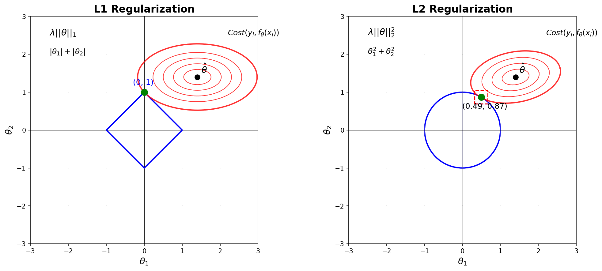
The key difference between L1 and L2 regularization lies in their geometry:
- L1 norm: \(|\theta_1| + |\theta_2| = c\) creates a diamond
- L2 norm: \(\theta_1^2 + \theta_2^2 = c\) creates a circle
Why These Shapes?🔗
L1 Diamond: The constraint \(|\theta_1| + |\theta_2| = c\) creates four linear boundaries:
- Quadrant I: \(\theta_1 + \theta_2 = c\) (slope = -1)
- Quadrant II: \(-\theta_1 + \theta_2 = c\) (slope = +1)
- Quadrant III: \(-\theta_1 - \theta_2 = c\) (slope = -1)
- Quadrant IV: \(\theta_1 - \theta_2 = c\) (slope = +1)
These connect at corners exactly on the axes at \((±c, 0)\) and \((0, ±c)\).
L2 Circle: The constraint \(\theta_1^2 + \theta_2^2 = c\) is simply a circle with radius \(\sqrt{c}\).
The Crucial Insight: Corners = Sparsity🔗
When we optimize: 1. Cost function contours expand from the unconstrained optimum 2. They first touch the constraint boundary 3. L1: Often hits at a corner → one parameter becomes exactly zero → sparse solution 4. L2: Hits smooth boundary → parameters shrink but stay non-zero → dense solution
Mathematical Details🔗
| Aspect | L1 (Lasso) | L2 (Ridge) |
|---|---|---|
| Penalty | \(\sum\|\theta_i\|\) | \(\sum\theta_i^2\) |
| Gradient | \(\text{sign}(\theta_i)\) | \(2\theta_i\) |
| Effect | Forces weights to 0 | Shrinks weights uniformly |
| Use when | Many irrelevant features | All features matter |
The gradient difference is key: - L1: Constant force regardless of weight size → can push to exactly zero - L2: Force proportional to weight → diminishes near zero
Implementation🔗
def regularization_loss(weights, reg_type='l2', lambda_reg=0.01):
    if reg_type == 'l1':
        return lambda_reg * sum(torch.abs(w).sum() for w in weights)
    elif reg_type == 'l2':
        return lambda_reg * sum((w**2).sum() for w in weights)
When to Use Which?🔗
L1 Regularization: - Feature selection needed - Interpretability important - Sparse data
L2 Regularization: - Multicollinearity present - Need stable predictions - All features relevant
Elastic Net combines both: \(\alpha\sum|\theta_i| + (1-\alpha)\sum\theta_i^2\)
Choosing λ🔗
- Small λ: Weak regularization → potential overfitting
- Large λ: Strong regularization → potential underfitting
- Find optimal λ: Use cross-validation
The constraint size scales as \(c = 1/\lambda\): - L1: Diamond vertices at \((±1/\lambda, 0)\) and \((0, ±1/\lambda)\) - L2: Circle radius = \(\sqrt{1/\lambda}\)
Summary🔗
L1 creates sparsity because its diamond constraint has corners on the axes.
L2 creates density because its circular constraint is smooth everywhere.
Choose based on your goal: feature selection (L1) or stable predictions (L2).