Lecture 03: Functions (Solutions)

Lecture 03: Functions (Solutions)#

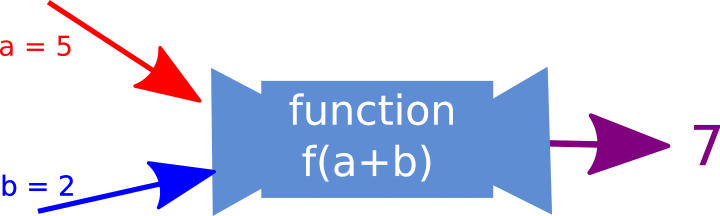
Exercise: Solution:

Functions are one of the most important concepts in computing. Similar to mathematical functions, they take input data and return an output(s). Functions are ideal for repetitive tasks that perform a particular operation on different input data and return a result. A simple function might take the coordinates of the vertices of a triangle and return the area. Any non-trivial program will use functions, and in many cases will have many functions.

Objectives#

Introduce construction and use of user functions
Returning from functions
Default arguments
Modules

functions

Purpose#

Functions allow computer code to be re-used multiple times with different input data. It is good to re-use code as much as possible because we then focus testing and debugging efforts, and maybe also optimisations, on small pieces of code that are then re-used. The more code that is written, the less frequently sections of code are used, and as a consequence the greater the likelihood of errors.

Functions can also enhance the readability of a program, and make it easier to collaborate with others. Functions allow us to focus on what a program does at a high level rather than the details of how it does it. Low-level implementation details are encapsulated in functions. To understand at a high level what a program does, we usually just need to know what data is passed into a function and what the function returns. It is not necessary to know the precise details of how a function is implemented to grasp the structure of a program and how it works. For example, we might need to know that a function computes and returns \(\sin(x)\); we don’t usually need to know how it computes sine.

Below is a simple example of a function being ‘called’ numerous times from inside a for loop.

import math
def approx_sin(x, tol):
    "Return an approximate sin value that depends on the input value x and tolerance"
    # Intialise approximation of sine
    sin = 0.0

    # Loop until error satisfies tolerance or a fixed number of iterations is reached
    for i in range(1001):
        sin+=(-1)**i*x**(2*i+1)/math.factorial(2*i+1)
        error=abs(sin-math.sin(x))
        if error<tol:
            return sin
            break
    else: #nobreak
        print("Error, sin(x) did not converge")



print("Case A: 3 values")
for y in range(3):
    print(y, approx_sin(y, 1e-3))

print("Case B: 12 values")
for y in range(12):
    print(y, approx_sin(y, 1e-6))

Case A: 3 values
0.0
0.8416666666666667
0.909347442680776
Case B: 12 values
0.0
0.8414710097001764
0.9092974515196738
0.14111965434119442
-0.7568025787396139
-0.9589238320910018
-0.27941540821600297
0.6569862528811284
0.9893581773748686
0.412118713523071
-0.5440217912423688
-0.9999903459807044

Using a function, we did not have to duplicate the sin computation inside each loop we re-used it. With a function we only have to change the way in which we calculate the sin of x in one place.

What is a function?#

Below is a Python function that takes two arguments (a and b), and returns a + b:

def sum(a, b):
    """"Return the sum of a and b"""
    return a + b

# Call the function
m = sum(3, 4)
print(m)  # Expect 7

# Call the function
m = 10
n = sum(m, m)
print(n)  # Expect 20

Using the above example as a model, we can examine the anatomy of a Python function.

A function is declared using def, followed by the function name, sum, followed by the list of arguments to be passed to the function between brackets, (a, b), and ended with a colon:
```
def sum(a, b):
```
Next comes the body of the function. The first part of the body is indented four spaces. Everything that makes up the body of the function is indented at least four spaces relative to def. In Python, the first part of the body is an optional documentation string that describes in words what the
function does
```
    "Return the sum of a and b"
```
It is good practice to include a ‘docstring’. What comes after the documentation string is the code that the function executes. At the end of a function is usually a return statement; this defines what result the function should return:
```
    return a + b
```

Anything indented to the same level (or less) as def falls outside of the function body.

Most functions will take arguments and return something, but this is not strictly required. Below is an example of a function that does not take any arguments or return any variables.

def print_message():
    print("The function 'print_message' has been called.")

print_message()

Function arguments#

The order in which function arguments are listed in the function declaration is in general the order in which arguments should be passed to a function.

For the function sum that was declared above, we could switch the order of the arguments and the result would not change because we are simply summing the input arguments. But, if we were to subtract one argument from the other, the result would depend on the input order:

def subtract(a, b):
    "Return a minus b"
    return a - b

alpha, beta = 3, 5  # This is short hand notation for alpha = 3
                    #                                 beta = 5

# Call the function and print the return value
print(subtract(alpha, beta))  # Expect -2
print(subtract(beta, alpha))  # Expect 2

For more complicated functions we might have numerous arguments. Consequently, it becomes easier to get the wrong order by accident when calling the function (which results in a bug). In Python, we can reduce the likelihood of an error by using named arguments, in which case order will not matter, e.g.:

print(subtract(a=alpha, b=beta))  # Expect -2
print(subtract(b=beta, a=alpha))  # Expect -2

-2
-2

Using named arguments can often enhance program readability and reduce errors.

What can be passed as a function argument?#

Many object types can be passed as arguments to functions, including other functions. Below is a function, is_positive, that checks if the value of a function \(f\) evaluated at \(x\) is positive:

def f0(x):
    "Compute x^2 - 1"
    return x*x - 1


def f1(x):
    "Compute -x^2 + 2x + 1"
    return -x*x + 2*x + 1

def is_f_p(f, x):
    if f(x) > 0:
        return True
    else:
        return False

print(is_f_p(f1, 0.5))

def is_positive(f, x):
    "Check if the function value f(x) is positive"

    # Evaluate the function passed into the function for the value of x
    # passed into the function
    if f(x) > 0:
        return True
    else:
        return False


# Value of x for which we want to test a function sign
x = 4.5

# Test function f0
print(is_positive(f0, x))

# Test function f1
print(is_positive(f1, x))

True
True
False

Default arguments#

It can sometimes be helpful for functions to have ‘default’ argument values which can be overridden. In some cases it just saves the programmer effort - they can write less code. In other cases it can allow us to use a function for a wider range of problems. For example, we could use the same function for vectors of length 2 and 3 if the default value for the third component is zero.

As an example we consider the position \(r\) of a particle with initial position \(r_{0}\) and initial velocity \(v_{0}\), and subject to an acceleration \(a\). The position \(r\) is given by:

\[ r = r_0 + v_0 t + \frac{1}{2} a t^{2} \]

Say for a particular application the acceleration is almost always due to gravity (\(g\)), and \(g = 9.81\) m s\(^{-1}\) is sufficiently accurate in most cases. Moreover, the initial velocity is usually zero. We might therefore implement a function as:

def position(t, r0, v0=0.0, a=-9.81):
    "Compute position of an accelerating particle."
    return r0 + v0*t + 0.5*a*t*t

# Position after 0.2 s (t) when dropped from a height of 1 m (r0)
# with v0=0.0 and a=-9.81
p = position(0.2, 1.0)
print(p)

0.8038

At the equator, the acceleration due to gravity is slightly less, and for a case where this difference is important we can call the function with the acceleration due to gravity at the equator:

# Position after 0.2 s (t) when dropped from a height of  1 m (r0)
p = position(0.2, 1, 0.0, -9.78)
print(p)

0.8044

Note that we have also passed the initial velocity - otherwise the program might assume that our acceleration was in fact the velocity. We can use the default velocity and specify the acceleration by using named arguments:

# Position after 0.2 s (t) when dropped from a height of  1 m (r0)
p = position(0.2, 1, a=-9.78)
print(p)

0.8044

Return arguments#

Most functions, but not all, return data. Above are examples that return a single value (object), and one case where there is no return value. Python functions can have more than one return value. For example, we could have a function that takes three values and returns the maximum, the minimum and the mean, e.g.

def compute_max_min_mean(x0, x1, x2):
    "Return maximum, minimum and mean values"

    x_min = x0
    if x1 < x_min:
        x_min = x1
    if x2 < x_min:
        x_min = x2

    x_max = x0
    if x1 > x_max:
        x_max = x1
    if x2 > x_max:
        x_max = x2

    x_mean = (x0 + x1 + x2)/3

    return x_min, x_max, x_mean


xmin, xmax, xmean = compute_max_min_mean(0.5, 0.1, -20)
print(xmin, xmax, xmean)

-20 0.5 -6.466666666666666

This function works, but we will see better ways to implement the functionality using lists or tuples in a later notebook.

Scope#

Functions have local scope, which means that variables that are declared inside a function are not visible outside the function. This is a very good thing - it means that we do not have to worry about variables declared inside a function unexpectedly affecting other parts of a program. Here is a simple example:

def f(x): # name x used as a formal parameter
    y = 1
    w = 2
    x = x + y + w
    print("x = ", x)
    return x

# Assign 3.0 to the variable x
x = 3.0
y = 2.0
print("x = ", x)
print("y = ", y)

z = f(x)
print("z = ", z)

# Check that the function declaration of 'x' has not affected
# the variable 'x' outside of the function
print("x = ", x)
print("y = ", y)

# This would throw an error - the variable c is not visible outside of the function
# print(w)

x =  3.0
y =  2
x =  6.0
z =  6.0
x =  3.0
y =  2

The variable x that is declared outside of the function is unaffected by what is done inside the function. Similarly, the variable w in the function is not ‘visible’ outside of the function.

There is more to scoping rules that we can skip over for now.

Recursion with functions#

A classic construction with functions is recursion, which is when a function makes calls to itself. Recursion can be very powerful, and sometimes also quite confusing at first. We demonstrate with a well-known example, the Fibonacci series of numbers.

Fibonacci number#

The Fibonacci series is defined recursively, i.e. the \(n\)th term \(f_{n}\) is computed from the preceding terms \(f_{n-1}\) and \(f_{n-2}\):

\[ f_n = f_{n-1} + f_{n-2} \]

for \(n > 1\), and with \(f_0 = 0\) and \(f_1 = 1\).

Below is a function that computes the \(n\)th number in the Fibonacci sequence using a for loop inside the function.

def fib(n):
    "Compute the nth Fibonacci number"
    # Starting values for f0 and f1
    f0, f1 = 0, 1

    # Handle cases n==0 and n==1
    if n == 0:
        return 0
    elif n == 1:
        return 1

    # Start loop (from n = 2)
    for i in range(2, n + 1):
        # Compute next term in sequence
        f = f1 + f0

        # Update f0 and f1
        f0 = f1
        f1 = f

    # Return Fibonacci number
    return f

print(fib(10))

Since the Fibonacci sequence has a recursive structure, with the \(n\)th term computed from the \(n-1\) and \(n-2\) terms, we could write a function that uses this recursive structure:

def f(n):
    "Compute the nth Fibonacci number using recursion"
    if n < 2:
        return n  # This doesn't call f, so it breaks out of the recursion loop
    else:
        return f(n - 1) + f(n - 2)  # This calls f for n-1 and n-2 (recursion), and returns the sum

print(f(10))

As expected (if the implementations are correct) the two implementations return the same result. The recursive version is simple and has a more ‘mathematical’ structure. It is good that a program which performs a mathematical task closely reflects the mathematical problem. It makes it easier to comprehend at a high level what the program does.

Care needs to be taken when using recursion that a program does not enter an infinite recursion loop. There must be a mechanism to ‘break out’ of the recursion cycle.

Modules#

So far, we have operated under the assumption that our entire program is stored in one file. This is perfectly reasonable as long as programs are small. As programs get larger, however, it is typically more convenient to store different parts of them in different files. Imagine, for example, that multiple people are working on the same program. It would be a nightmare if they were all trying to update the same file. Python modules allow us to easily construct a program from code in multiple files.

A module is a .py file containing Python definitions and statements. We could create, for example, a file circle.py containing:

pi = 3.14159

def area(radius):
    return pi*(radius**2)

def circumference(radius):
    return 2*pi*radius

def sphereSurface(radius):
    return 4.0*area(radius)

def sphereVolume(radius):
    return (4.0/3.0)*pi*(radius**3)

A program gets access to a module through an import statement. So, for example, the code

# Import Google Drive and mount google drive volume to Jupyter notebook
from google.colab import drive
drive.mount('/content/gdrive')
!ls '/content/gdrive/My Drive/CE311K/lectures/03_functions'
# Add Google drive path to locate modules
import sys
sys.path.append('/content/gdrive/My Drive/CE311K/lectures/03_functions')
print(sys.path)

import circle
print(circle.pi)
print(circle.area(3))
print(circle.circumference(3))
print(circle.sphereSurface(3))

14159
27431
849539999999998
09724