Lecture 10: Useful libraries in Python (Solution)

Exercise: Solution:

• Sympy (Symbolic notations)

• Scipy (optimize)

• Fsolve (Linear and Nonlinear equations)

• Curve fitting

Solving ordinary differential equations

Sympy to solve some ODE examples. To use Sympy, we first need to import it and call init_printing() to get nicely typeset equations

import sympy
from sympy import symbols, Eq, Derivative, init_printing, Function, dsolve, exp, classify_ode, checkodesol

# This initialises pretty printing
init_printing()
from IPython.display import display

# Support for interactive plots
from ipywidgets import interact

# This command makes plots appear inside the browser window
%matplotlib inline

Example: car breaking

During braking a car’s velocity is given by \(v = v_{0} e^{−t/\tau}\). Calculate the distance travelled.

We first define the symbols in the equation (\(t\), \(\tau\) and \(v_{0}\)), and the function (\(x\), for the displacement):

\[\frac{d x(t)}{dt} = v_{0} e^{−t/\tau} \quad \rightarrow \quad x(t) = \int v_{0} e^{−t/\tau} dt\]

t, tau, v0 = symbols("t tau v0")
x = Function("x")

Next, we define the differential equation, and print it to the screen for checking:

eqn = Eq(Derivative(x(t), t), v0*exp(-t/(tau)))
display(eqn)

The dsolve function solves the differential equation symbolically:

x = dsolve(eqn, x(t))
display(x)

where \(C_{1}\) is a constant. As expected for a first-order equation, there is one constant.

SymPy is not yet very good at eliminating constants from initial conditions, so we will do this manually assuming that \(x = 0\) and \(t = 0\):

x = x.subs('C1', v0*tau)
display(x)

Specifying a value for \(v_{0}\), we create an interactive plot of \(x\) as a function of the parameter \(\tau\):

x = x.subs(v0, 100)

def plot(τ=1.0):
    x1 = x.subs(tau, τ)

    # Plot position vs time
    sympy.plot(x1.args[1], (t, 0.0, 10.0), xlabel="time", ylabel="position");

interact(plot, τ=(0.0, 10, 0.2));

Scipy Optimize

Bisection

Find root of a function within an interval using bisection.

Basic bisection routine to find a zero of the function f between the arguments a and b. f(a) and f(b) cannot have the same signs.

from scipy import optimize

# Define a function
def f(x):
    return (x**2 - 1)

root = optimize.bisect(f, 0, 2)
print("The root of the function: {}".format(root))

The root of the function: 1.0

Newton Raphson

Find a zero of the function func given a nearby starting point x0.

from scipy import optimize

# Define a function
def f(x):
    return (x**3 - 1)  # only one real root at x = 1

root = optimize.newton(f, 1.5)
print("The root of the function: {}".format(root))

The root of the function: 1.0000000000000016

Systems of equations

Linear equations

System of m equations \((i = 1, \dots, m)\) in \(n\) unknowns \(x_j \quad (j = 1, \dots, n)\) can be represented as \(Ax = b\). For example,

\[\begin{split} \begin{align*} x_1 + 2 x_2 & = 5\\ -3 x_1 + 4 x_2 & = 20 \\ \end{align*} \end{split}\]

\[\begin{split} Ax = b \rightarrow \begin{bmatrix} 1 & 2 \\ -3 & 4 \\ \end{bmatrix} \begin{bmatrix} x_1 \\ x_2 \\ \end{bmatrix}= \begin{bmatrix} 5 \\ 20 \\ \end{bmatrix} \end{split}\]

To solve a linear system of equations, we will use numpy.linalg.solve, which requires a matrix \(A\) and a vector \(b\) as arguments.

import numpy as np

# Define the matrix A and vector b
A = np.array([[1, 2], [-3, 4]])
b = np.array([5, -20])

# Solve the system of linear equations
x = np.linalg.solve(A, b)
print("The solution x: {}".format(x))

The solution x: [ 6.  -0.5]

Non-linear equations

Solving a system of non-linear equations:

\[\begin{split} \begin{align*} x_1 + x_2^2 & = 4\\ e^{x_1} + x_1 x_2 & = 3 \\ \end{align*} \end{split}\]

We need to rearrange each equation such that we have 0 on the right-hand side.

\[\begin{split} \begin{align*} f_1(x) = x_1 + x_2^2 -4 & = 0\\ f_2(x) = e^{x_1} + x_1 x_2 -3 & = 0 \\ \end{align*} \end{split}\]

Non-linear system of equations can be solved using scipy.optimize.fsolve

from scipy.optimize import fsolve
import math

# z is a vector collecting x1 and x2
def equations(z):
    x1, x2 = z
    return (x1+x2**2 -4, math.exp(x1) + x1 * x2 - 3)

x1, x2 = fsolve(equations, (1, 1))

print("x1 is {:.3f}, x2 is {:.3f}".format(x1, x2))
print("Check if the solution for f(z) = 0")
print(equations((x1, x2)))

x1 is 0.620, x2 is 1.838
Check if the solution for f(z) = 0
(4.4508396968012676e-11, -1.0512035686360832e-11)

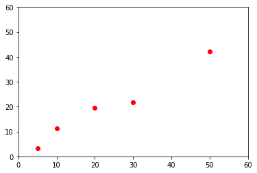
Curve fitting

Linear and polynomial fits with np.polyfit

import numpy as np
import matplotlib.pyplot as plt

x = np.array([5, 10,20,30,50]) 
y = np.array([3.3, 11.2, 19.5, 21.8, 42.3])

plt.plot(x, y, 'or')
plt.axis([0 , 60, 0 , 60])

plt.show()

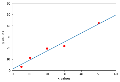
# Fit a straight line through points
x = np.array([5, 10,20,30,50]) 
y = np.array([3.3, 11.2, 19.5, 21.8, 42.3])

# coefficients
coeffs = np.polyfit(x, y, 1)
polynomial = np.poly1d(coeffs)

print("The polynomial is: {}".format(polynomial))
print("Regression coefficients are: {}".format(coeffs))

The polynomial is:  
0.8056 x + 1.091
Regression coefficients are: [0.805625 1.090625]

# Plot the fit
xp = np.linspace(0,60,100)

plt.plot(x, y, 'or', xp, polynomial(xp), '-')
plt.axis([0 , 60, 0 , 60])
plt.xlabel('x values')
plt.ylabel('y values')

plt.show()

# Fit a cubic polynomial
x = np.array([5, 10,20,30,50]) 
y = np.array([3.3, 11.2, 19.5, 21.8, 42.3])

# coefficients
coeffs = np.polyfit(x, y, 3)
polynomial = np.poly1d(coeffs)

# Plot the fit
xp = np.linspace(0,60,100)

plt.plot(x, y, 'or', xp, polynomial(xp), '-')
plt.axis([0 , 60, 0 , 60])
plt.xlabel('x values')
plt.ylabel('y values')

plt.show()

print(polynomial)

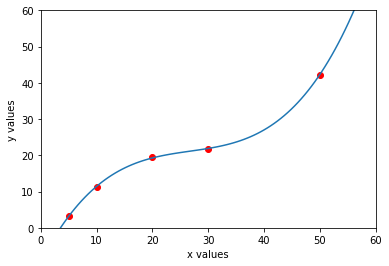
          3          2
0.001282 x - 0.1029 x + 2.973 x - 9.272