Kernels, Families of Functions, and Shapes That Move🔗
So far, the function is known and the question is how well a finite representation approximates it. For a cooling fin, only noisy temperature measurements are available. The unknown curve must now be inferred from those measurements and assumptions about its variation.
Reconstructing temperature from scattered measurements🔗
Consider thermocouples measuring temperature at fixed locations along a cooling fin. Let \(x \in [0,1]\) denote normalized distance along the fin, and let \(y_i\) be the reading at \(x_i\). The readings constrain the temperature at the sensors, but leave infinitely many possible curves between them. How should a reading influence the estimate at a neighboring location?
Heat conduction motivates a smooth temperature profile. Nearby locations should have similar temperatures, with less agreement expected as their separation grows. The squared-exponential kernel expresses this assumption through
Here \(\ell\) sets the distance over which the similarity decreases. It is a parameter of the representation, whose suitability must be checked against the measurements. A short length scale permits rapid variation, while a long one favors gradual variation.
A copy of this kernel centered at a sensor is a smooth function of position. A weighted sum of the copies gives the temperature estimate,
Each weight determines how much its copy contributes to the reconstructed curve. Because neighboring copies overlap, their weights generally differ from the readings. The weights must be chosen together.
To interpolate the readings, evaluate the sum at each sensor and require \(\hat f(x_i)=y_i\). With \(K_{ij}=k(x_i,x_j)\), these equations form the linear system
For distinct sensor locations, the squared-exponential kernel gives a symmetric positive-definite matrix. The interpolation weights are therefore unique. This guarantee concerns agreement at the sensors, not accuracy between them.
For a hand calculation, take two sensors separated by \(\ell\), each with reading one. Their similarity is \(\rho=e^{-1/2}\), and symmetry gives equal weights \(\alpha\). At either sensor, the sum is \(\alpha+\rho\alpha=1\), so each weight is \(1/(1+\rho)\). The contribution from the neighboring copy reduces the weight needed at that sensor.
The interactive figure uses synthetic fin measurements, so a reference profile is available for comparison. At \(\ell=0.15\), the interpolant at \(x=0.7\) is \(0.216\), against the reference value \(0.393\). At \(\ell=0.04\), the estimate there is below \(0.001\), although every sensor reading is still reproduced. Agreement at the sensors alone does not validate the length scale.
When a similarity defines an inner product🔗
The similarity between two locations should also describe the inner product of their kernel copies. An arbitrary similarity rule need not support such an interpretation. Consider a rule that assigns one to locations less than \(\ell\) apart and zero otherwise. At the sites \(0\), \(0.6\ell\), and \(1.2\ell\), it gives
For the weights \(\mathbf{w}=(1,-\sqrt{2},1)^\top\), the quadratic form is \(\mathbf{w}^\top\mathbf{K}\mathbf{w}=4-4\sqrt{2}<0\). If the entries were inner products, this value would be the squared norm of a weighted sum. A squared norm cannot be negative, so this rule fails.
A symmetric kernel is positive definite when every finite choice of sites and weights gives a nonnegative quadratic form. Here the convention permits zero, so the associated matrices are positive semidefinite. Strict positive definiteness requires a positive value for nonzero weights at distinct sites. The squared-exponential kernel satisfies this stronger condition.
A kernel constructed from feature vectors \(\Phi(x)\) has the required nonnegativity. If \(k(x,x')=\langle\Phi(x),\Phi(x')\rangle\), then
The feature vectors may belong to an infinite-dimensional inner-product space. A positive-definite kernel admits such a feature representation, even when the features are not written explicitly. What function space does this inner product define?
Point evaluation in a kernel space🔗
For the squared-exponential kernel, a single copy has squared norm \(k(x_i,x_i)=1\). Copies centered at \(x_1\) and \(x_2\) have inner product \(\rho=k(x_1,x_2)\). Their sum has squared norm \(2+2\rho\), while their difference has squared norm \(2-2\rho\). Thus nearby copies are close in this norm.
These calculations extend to every finite weighted sum by linearity. Their Cauchy sequences have terms that become arbitrarily close in this norm. Completing the sums includes the limits of those sequences. The resulting function space is the reproducing kernel Hilbert space \(\mathcal{H}_k\). Its inner product satisfies
This inner product differs from the integral of the product of two kernel copies. Its geometry is specified by the kernel values themselves. The norm in this geometry is denoted by \(\|f\|_k\).
To evaluate a weighted sum \(f\), take its inner product with the copy centered at the evaluation point. For \(f=\alpha_1k(x_1,\cdot)+\alpha_2k(x_2,\cdot)\), linearity gives \(\alpha_1k(x_1,x)+\alpha_2k(x_2,x)\). This expression is the value \(f(x)\). The same identity extends to every member of \(\mathcal{H}_k\),
The Cauchy-Schwarz inequality therefore bounds each point value by \(|f(x)|\leq\|f\|_k\sqrt{k(x,x)}\). For the squared-exponential kernel, \(k(x,x)=1\), so closeness in the RKHS norm implies closeness at every point. This makes point readings well-defined and continuous, which the \(L^2\) norm alone does not provide.
For this differentiable kernel, the reproducing identity also gives the slope bound \(|f'(x)|\leq\|f\|_k/\ell\). A function that increases by one over a distance \(\ell/10\) must have a slope of at least \(10/\ell\) somewhere, so its RKHS norm is at least ten. The norm constrains both amplitude and variation. How can this constraint help when the readings contain noise?
Fitting noisy measurements🔗
Interpolation reproduces the noise along with the measured temperature. The effect can be large when nearby kernel copies are nearly dependent. For two sensors with similarity \(\rho=0.99\), the matrix eigenvalues are \(1+\rho=1.99\) and \(1-\rho=0.01\). They correspond to equal and opposite changes in the readings.
Opposite measurement errors \((\varepsilon,-\varepsilon)\) change the interpolation weights by \((100\varepsilon,-100\varepsilon)\). The difference of the two kernel copies has RKHS norm \(\sqrt{2-2\rho}\). Thus the reconstructed function changes by approximately \(14.1|\varepsilon|\) in RKHS norm. Large coefficient changes and large function changes are related, but their magnitudes differ.
A regularized fit permits disagreement with noisy readings and penalizes the RKHS norm. For \(\lambda>0\), kernel ridge regression minimizes
The first term measures squared disagreement at the sensors. The second discourages the amplitude and variation needed to fit every fluctuation. The parameter \(\lambda\) determines their relative importance.
Any component orthogonal to the span of the sensors' kernel copies has zero value at every sensor. It changes none of the fitting errors and increases the norm, so the minimizer has no such component. The fit therefore remains a weighted kernel sum, with weights satisfying
Adding \(\lambda\) to each eigenvalue reduces the amplification caused by small eigenvalues. In the two-sensor example, \(\lambda=0.1\) changes the small divisor from \(0.01\) to \(0.11\). The coefficient amplification falls from \(100\) to approximately \(9.1\). Can the same kernel also describe uncertainty between the sensors?
Uncertainty from a Gaussian process🔗
A temperature at an unmeasured location can be described by a probability distribution. To see how a measurement changes that distribution, take independent standard Gaussian variables \(Z_1\) and \(Z_2\). Define temperatures at two locations by
Both temperatures have mean zero and variance one, with covariance \(\rho\). Observing \(f(x_1)=y\) fixes \(Z_1=y\). The remaining temperature has conditional mean \(\rho y\) and standard deviation \(\sqrt{1-\rho^2}\). Stronger correlation gives less remaining uncertainty.
A Gaussian process extends this construction to any finite collection of locations. Assume a zero prior mean and covariance \(k(x,x')\). The measured values are \(y_i=f(x_i)+\varepsilon_i\), with independent Gaussian noise of variance \(\sigma^2\). For \(\mathbf{k}_x=(k(x,x_1),\ldots,k(x,x_m))^\top\), conditioning gives
The posterior mean \(m\) equals the kernel ridge fit with \(\lambda=\sigma^2\) for the unnormalized squared-error objective above. The posterior variance \(v\) measures remaining uncertainty about the latent temperature, rather than a future noisy measurement. The subtracted term is the reduction in variance supplied by the sensors.
The shaded band is \(m(x)\pm2\sqrt{v(x)}\), conditional on the selected kernel and noise model. With noise standard deviation \(0.03\), its largest half-width in the unsensed stretch is \(0.90\) at \(\ell=0.15\) and \(1.99\) at \(\ell=0.075\). Shorter-range correlations leave greater uncertainty between the sensors. These are pointwise posterior bands, without a guarantee of simultaneous coverage of the whole curve.
The marginal likelihood scores how well a kernel and noise model explain the observed readings. Maximizing it over the tested length scales gives \(\ell=0.31\) in this synthetic experiment. The resulting mean has relative \(L^2\) error \(3.2\) percent, and the maximum band half-width in the gap is \(0.12\). These results depend on the model assumptions, which must be reconsidered if the temperature has a sharp transition.
A moving front gives a family of functions🔗
Now consider a hot region transported along a pipe. For constant flow speed \(c\) and negligible diffusion, its temperature profile translates without changing shape. At each time, the profile is a function of position on the same interval. The reconstruction must describe the hot region wherever it moves.
The figure below shows the hot region in the pipe, its temperature profiles, and their reconstructions on one fixed grid. The edges move to new locations, while the grid nodes remain in place. The reconstruction joins the temperature values at those nodes with straight segments.
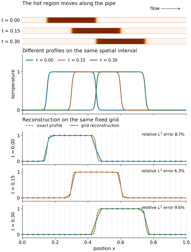
The plotted profile has transition width \(w=0.01\) and moves at normalized speed \(c=1\). The fixed grid has \(32\) nodes, with spacing \(1/31\). At times \(0\), \(0.15\), and \(0.30\), its relative \(L^2\) reconstruction errors are \(8.7\), \(6.3\), and \(9.6\) percent. The same grid represents some edge locations more accurately than others.
Let \(T_0\) denote the initial profile. Translation gives the profile at time \(t\),
Each time selects a different function of \(x\), while \(T_0\) and \(c\) remain fixed. The collection \(\mathcal{S}=\{T_0(\cdot-ct)\mid 0\leq t\leq0.30\}\) is a family parameterized by time. Knowing the initial shape and the translation rule specifies every member from that parameter.
A fixed-grid representation uses hat functions \(\phi_i\) centered at nodes \(x_i\). Only their coefficients change with time,
Every reconstructed profile therefore belongs to the same linear span of the hats. Many nodes are needed when the edge width is small compared with their spacing. The moving-nodes lab instead places its breakpoints near the edges. Does choosing a different fixed basis remove this difficulty for the whole family?
The limits of a fixed linear space🔗
A narrow pulse centered at separated locations gives profiles with little overlap. The finite-dimensional version is a unit spike translated across three grid points. Its snapshots are the perpendicular vectors \(\mathbf{e}_1\), \(\mathbf{e}_2\), and \(\mathbf{e}_3\) in \(\mathbb{R}^3\). These snapshots provide a calculation that applies to every plane through the origin.
Let \(P\) be the orthogonal projection onto such a plane. The squared projection lengths add to the plane's dimension, so the squared errors satisfy
At least one error is therefore no smaller than \(1/\sqrt{3}\). No choice of the plane can approximate all the snapshots more closely than this bound in Euclidean norm. Exact linear representation of the snapshots requires dimension three, although one position parameter selects the spike.
For a family of functions, the Kolmogorov \(n\)-width asks how well the best fixed \(n\)-dimensional linear space approximates its worst member. Using the \(L^2\) norm, it is
The inner infimum chooses the closest member of \(V\) for each target. The supremum chooses the hardest target in the family, and the outer infimum chooses the space. The space must be chosen once for the entire family.
Motion alone does not imply a large width. Every translate of \(\sin(kx)\) lies in the span of \(\sin(kx)\) and \(\cos(kx)\) by the angle-subtraction identity. A localized pulse with steep edges instead requires many frequencies, and translation does not reduce their magnitudes. For a periodic heat equation with unit diffusivity, those magnitudes decay by \(e^{-(2\pi k)^2t}\), explaining why diffusion can reduce the required number of modes.
A snapshot matrix's singular value decomposition minimizes average squared projection error over the sampled profiles. The width concerns the worst profile over the entire family. A small average error on snapshots therefore needs a separate check of poorly represented positions. Can the representation adapt to the target instead of using one fixed linear space?
Representations that adapt to the front🔗
The translated-template formula already gives an alternative to fixed-grid coefficients. It stores the initial shape and evaluates that shape at shifted coordinates. This representation assumes a known translation law, but its functions need not belong to one low-dimensional linear space. Other adaptive representations change their locations, shapes, or selected terms.
Move the locations with the flow🔗
A particle representation stores positions together with temperature values. For pure advection, each particle keeps its temperature while its position follows the flow. The field between particles is reconstructed from their values and an interpolation rule. Exact transport of stored values does not remove this reconstruction error.
A first-order upwind grid scheme provides a useful comparison. For positive speed and \(0<\nu=c\Delta t/h<1\), its update is
Each step averages neighboring temperatures, which spreads a steep transition. This numerical diffusion comes from the update rule, separately from the fixed basis's approximation error. At \(\nu=1\), the update shifts grid values without averaging.
Fit the locations and shapes🔗
A Gaussian element describes a localized field through its center, covariance, and amplitude. An anisotropic covariance permits a long, narrow shape aligned with a ridge. Fitting these parameters lets the elements concentrate where the field varies. The Gaussian-field figure illustrates the reconstruction as elements are added and their widths change.
With centers and covariances fixed, a quadratic fitting objective gives a linear system for the amplitudes. Fitting the centers and covariances as well generally makes the objective non-convex. The representation can adapt to localized features, but the fitting algorithm may stop at a poor local minimum.
Select localized terms🔗
A wavelet representation keeps its dictionary fixed and selects terms for each profile. For an orthonormal Haar expansion, retaining the \(n\) largest coefficients minimizes the \(L^2\) truncation error among selections of \(n\) terms. For a front, the selected terms tend to be concentrated near the edges. As the edges move, different terms are selected.
The selected functions belong to different dictionary subspaces, so the width's fixed-space restriction no longer describes this approximation. Storage must include the selected indices as well as the coefficient values. Resolution and truncation still limit accuracy, so adapting the selection does not guarantee a good reconstruction.
Choosing a representation for the fin🔗
For the fin, the unknown profile must be reconstructed from the same noisy measurements. The synthetic reference permits a direct comparison, but such a reference is unavailable in practice. The table compares relative \(L^2\) error against that reference with prediction error obtained by withholding readings.
| Representation and fitting principle | Relative \(L^2\) error against reference | Held-out RMSE |
|---|---|---|
| Straight segments | \(6.5\%\) | \(0.095\) |
| Cubic polynomial, least squares | \(23\%\) | \(0.310\) |
| Polynomial interpolation | \(31\%\) | \(3.57\) |
| Kernel interpolation, \(\ell=0.15\) | \(11\%\) | \(0.112\) |
| Gaussian-process mean, \(\ell=0.31\) | \(3.2\%\) | \(0.034\) |
The held-out calculation removes each reading, fits the remaining readings, and predicts the omitted value. Its RMSE is measured in the normalized temperature units, against noise standard deviation \(0.03\). The length scales remain fixed at values selected using all the readings, so this is a fixed-hyperparameter diagnostic. Testing the complete selection procedure requires choosing the length scale again within each fold.
The table favors the Gaussian-process fit in this experiment, without establishing that it is best for every fin. The kernel specifies the possible functions and their geometry, while regularized fitting selects a function using the measurements. The posterior band adds uncertainty conditional on the same assumptions. The comparison below records the assumptions that should be checked for each representation.
For a moving front, a reconstruction must also be checked across its possible positions. A low-dimensional parameterization can describe a family that is difficult for one small fixed linear space. Choosing a representation therefore requires both a reconstruction rule and a clear statement of which functions it must approximate.
The companion notebooks on the cooling fin and one front, every family contain the underlying experiments. The fin notebook compares interpolation, regularization, and uncertainty from the same measurements. The front notebook compares fixed and adaptive representations of the transported profile.