12: Graph Neural Network

Exercise: Solution:

Setup

The installation of PyG on Colab can be a little bit tricky. Before we get started, let’s check which version of PyTorch you are running.

import os
import torch
print(f"PyTorch has version {torch.__version__} with cuda {torch.version.cuda}")

Download the necessary packages for PyG. Make sure that your version of torch matches the output from the cell above. In case of any issues, more information can be found on PyG’s installation page

# Install torch geometric
!pip install torch-cluster -f https://data.pyg.org/whl/torch-2.1.0+cu118.html
!pip install torch-scatter -f https://data.pyg.org/whl/torch-2.1.0+cu118.html
!pip install torch-sparse -f https://data.pyg.org/whl/torch-2.1.0+cu118.html
!pip install torch-geometric

Graph Neural Networks (GNNs) and message passing

Although traditional physics simulators are powerful, there are some important drawbacks with them: (1) it is expensive and time-consuming to get high-quality results of large-scale simulations for traditional physical simulators; (2) to set up physical simulators, we need to have full knowledge of the physics parameters of the object and the environment, which are extremely hard to know in some cases.

Graph Neural Network (GNN) is a special subset of neural networks that take less structured data, such as a graph, as input, while other neural networks like Convolutional Neural Network (CNN) and Transformer, can only accept more structured data (e.g., grid and sequence). By “less structured”, it means that the input can have arbitrary shapes and sizes and can have complex topological relations.

In particle-based physics simulation, we have the unstructured position information of all the particles as the input, which inspires the idea of using a GNN.

Permutation equivariance

One key characteristic of GNN which distinguishes it from other neural networks is permutation equivalence. That is to say, the nodes in a graph do not have a canonical order, so how we “order” the nodes in a graph does not impact the results produced by GNNs.

Since particles of an object are “identical” in the particle-based simulation, they are permutation-equivariant when applying physics laws on them. Therefore, a permutation-equivariant model such as a GNN is suitable to simulate the interactions between particles.

Graphs

Graphs are powerful means of representing interactions between physical systems. A granular material media can be represented as a graph \( G=\left(V,E\right) \) consisting of a set of vertices (\(\mathbf{v}_i \in\ V\)) representing the soil grains and edges (\(\mathbf{e}_{i,j} \in\ E\)) connecting a pair of vertices (\(\mathbf{v}_i\) and \(\mathbf{v}_j\)) representing the interaction relationship between grains. We describe how graphs work by showing a simple example involving interaction between balls in a box (Figure 1a). The state of the physical system (Figure 1a and 1d) can be encoded as a graph (Figure 1b and 1c). The vertices describe the balls, and the edges describe the directional interaction between them, shown as arrows in Figure 1b and 1c. The state of the ball i is represented as a vertex feature vector \(\mathbf{v}_i\) at \(i\). The feature vector includes properties such as velocities, mass, and distance to the boundary. The edge feature vector \(\mathbf{e}_{i,j}\) includes the information about the interaction between balls \(i\) and \(j\) such as the relative distance between the balls.

Graphs offer a permutation invariant form of encoding data, where the interaction between vertices is independent of the order of vertices or their position in Euclidean space. Rather, graphs represent the interactions through the edge connection, not affected by the permutation of the vertices. Therefore, graphs can efficiently represent the physical state of granular flow where numerous orderless particles interact by using vertices to represent particles and edges to their interaction.

Graph neural networks (GNNs)

GNNs are a state-of-the-art deep learning architecture that can operate on a graph and learn the local interactions. GNNs take a graph \(G=\left(\mathbf{V},\mathbf{E}\right)\) at time t as an input, compute properties and propagate information through the network, termed as message passing, and output an updated graph \(G^\prime=\left(\mathbf{V}^\prime,\mathbf{E}^\prime\right)\) with an identical structure, where \(\mathbf{V}^\prime\) and \(\mathbf{E}^\prime\) are the set of updated vertex and edge features (\(\mathbf{v}_i^\prime\) and \(\mathbf{e}_{i,\ j}^\prime\)). In the balls-in-a-box example, the GNN first takes the original graph \(G=\left(\mathbf{V},\mathbf{E}\right)\) (Figure 1b) that describes the current state of the physical system (\(\mathbf{X}^t\)). The GNN then updates the state of the physical system through message passing, which models the exchange of energy and momentum between the balls communicating through the edges, and returns an updated graph \(G^\prime=\left(\mathbf{V}^\prime,\mathbf{E}^\prime\right)\) (Figure 1c). After the GNN computation, we may decode G^\prime to extract useful information related to the future state of the physical system (\(\mathbf{X}^{t+1}\)) such as the next position or acceleration of the balls (Figure 1d).

Figure. 1. An example of a graph and graph neural network (GNN) that process the graph (modified from Battaglia et al. (2018)): (a) A state of the current physical system (\(\mathbf{X}^t\)) where the balls are bouncing in a box boundary; (b) Graph representation of the physical system (\(G\)). There are three vertices representing balls and six edges representing their directional interaction shown as arrows; (c) The updated graph (\(G^\prime\)) that GNN outputs through message passing; (d) The predicted future state of the physical system (\(\mathbf{X}^{t+1}\)) (i.e., the positions of the balls at the next timestep) decoded from the updated graph.

Message passing

Message passing consists of three operations: message construction (Eq. 1), message aggregation (Eq. 2), and the vertex update function (Eq. 3).

\[ \begin{equation} \mathbf{e}_{i,j}^\prime=\phi_{\mathbf{\Theta}_\phi}\left(\mathbf{v}_i,\mathbf{v}_j,\mathbf{e}_{i,\ j}\right) \end{equation} \]

\[ \begin{equation} {\bar{\mathbf{v}}}_i=\Sigma_{j \in N\left(i\right)}\ \mathbf{e}_{i,j}^\prime \end{equation} \]

\[ \begin{equation} \mathbf{v}_i^\prime=\gamma_{\mathbf{\Theta}_\gamma}\left(\mathbf{v}_i,{\bar{\mathbf{v}}}_i\right) \end{equation} \]

The subscript \(\mathbf{\Theta}_\phi\) and \(\mathbf{\Theta}_\gamma\) represent a set of learnable parameters in each computation. The message construction function \(\phi_{\Theta_{\phi}}\) (Eq. 1) takes the feature vector of the receiver and sender vertices (\(\mathbf{v}_i\) and \(\mathbf{v}_j\)) and the feature vector of the edge connecting them (\(\mathbf{e}_{i,\ j}\)) and returns an updated edge feature vector \(\mathbf{e}_{i,j}^\prime\) as the output. \(\phi_{\Theta_{\phi}}\) is a matrix operation including the learnable parameter \(\mathbf{\Theta}_\phi\). The updated edge feature vector \(\mathbf{e}_{i,j}^\prime\) is the message sent from vertex \(j\) to \(i\). Figure 2a shows an example of constructing messages on edges directing to vertex 0 originating from vertices 1, 2, and 3 (\(\mathbf{e}_{0,1}^\prime, \mathbf{e}_{0,2}^\prime, \mathbf{e}_{0,3}^\prime\)). Here, we define the message construction function \(\phi_{\Theta_{\phi}}\) as \(\left(\left(\mathbf{v}_i+\mathbf{v}_j\right)\times\mathbf{e}_{i,j}\right)\times\mathbf{\Theta}_\phi\). The updated feature vector \(\mathbf{e}_{0,\ 1}^\prime\) is computed as \(\left(\left(\mathbf{v}_0+\mathbf{v}_1\right)\times\mathbf{e}_{0,1}\right)\times\mathbf{\Theta}_\phi\), where \(\mathbf{v}_0\) and \(\mathbf{v}_1\) are the receiver and sender vertex feature vectors, and \(\mathbf{e}_{0,1}\) is their edge feature vector. If we assume that all values of \(\mathbf{\Theta}_\phi\) are 1.0 for simplicity, we obtain \(\mathbf{e}_{0,\ 1}^\prime=(\left(\left[1,\ 0,\ 2\right]\right)+\left[1,\ 3,\ 2\right])\times\left[2,\ 1,\ 0\right]^T)\times1=[4,\ 3,\ 0]\). Similarly, we compute the messages \(\mathbf{e}_{0,\ 2}^\prime=\left[0,\ 3,\ 9\right]\) and \(\mathbf{e}_{0,\ 3}^\prime=\left[3,\ 4,\ 9\right]\).

The next step in message passing is the message aggregation \(\Sigma_{j \in N\left(i\right)}\) (Eq. 2), where \(N\left(i\right)\) is the set of sender vertices j related to vertex \(i\). It collects all the messages directing to vertex \(i\) and aggregates those into a single vector with the same dimension as the aggregated message (\({\bar{\mathbf{v}}}_i\)). The aggregation rule can be element-wise vector summation or averaging, hence it is a permutation invariant computation. In Figure 2a, the aggregated message \(\bar{\mathbf{v}_0}=\left[7,10,18\right]\) is the element-wise summation of the messages directing to vertex 0 as \(\bar{\mathbf{v}_o}=\mathbf{e}_{0,\ 1}^\prime+\ \mathbf{e}_{0,\ 2}^\prime+\ \mathbf{e}_{0,\ 3}^\prime\).

The final step of the message passing is updating vertex features using Eq. 3. It takes the aggregated message (\({\bar{\mathbf{v}}}_i\)) and the current vertex feature vector \(\mathbf{v}_i\), and returns an updated vertex feature vector \(\mathbf{v}_i^\prime\), using predefined vector operations including the learnable parameter \(\mathbf{\Theta}_\gamma\). Figure 2b shows an example of the update at vertex 0. Here, we define the update function \(\gamma_{\Theta_{\gamma}}\) as \(\mathbf{\Theta}_\gamma\left(\mathbf{v}_i+{\bar{\mathbf{v}}}_i\right)\). The updated feature vector \(\mathbf{v}_0^\prime\) is computed as \(\mathbf{\Theta}_\gamma\left(\mathbf{v}_0+{\bar{\mathbf{v}}}_\mathbf{0}\right)\). Assuming all parameters in \(\mathbf{\Theta}_\gamma\) are 1.0 for simpliticy, we obtain \(\mathbf{v}_0^\prime=\left[1,\ 0,\ 2\right]+\left[7,\ 10,\ 18\right]=\left[8,10,20\right]\). Similarly, we update the other vertex features \((\mathbf{v}_1^\prime, \mathbf{v}_2^\prime, \mathbf{v}_3^\prime)\).

At the end of the message passing, the graph vertex and edge features (\(\mathbf{v}_i\) and \(\mathbf{e}_{i,\ j}\)) are updated to \(\mathbf{v}_i^\prime\) and \(\mathbf{e}_{i,\ j}^\prime\). The GNN may include multiple message passing steps to propagate the information further through the network.

{width=55%} (a) {width=55%} (b)

Figure 2. An example of message passing on a graph: (a) message construction directing to receiver vertex 0 \((\mathbf{e}_{0,\ 1}^\prime, \mathbf{e}_{0,\ 2}^\prime, \mathbf{e}_{0,\ 3}^\prime)\) and the resultant aggregated message \(({\bar{\mathbf{v}}}_0)\); (b) feature update at vertex 0 using \({\bar{\mathbf{v}}}_0\). Note that we assume \(\mathbf{\Theta}_\phi\) and \(\mathbf{\Theta}_r\) are 1.0 for the convenience of calculation.

Unlike the example shown above, where we assume a constant value of 1.0 for the learnable parameters, in a supervised learning environment, the optimization algorithm will find a set of the best learnable parameters (\(\mathbf{\Theta}_\phi, \mathbf{\Theta}_\gamma\)) in the message passing operation.

Graph Neural Network-based Simulator (GNS)

In this study, we use GNN as a surrogate simulator to model granular flow behavior. Figure 3 shows an overview of the general concepts and structure of the GNN-based simulator (GNS). Consider a granular flow domain represented as particles (Figure 3a). In GNS, we represent the physical state of the granular domain at time t with a set of \(\mathbf{x}_i^t\) describing the state and properties of each particle. The GNS takes the current state of the granular flow \(\mathbf{x}_t^i \in \mathbf{X}_t\) and predicts its next state \({\mathbf{x}_{i+1}^i \in\ bm{X}}_{t+1}\) (Figure 3a). The GNS consists of two components: a parameterized function approximator \(\ d_\mathbf{\Theta}\) and an updater function (Figure 3b). The approximator \(d_\theta\) take takes \(\mathbf{X}_t\) as an input and outputs dynamics information \({\mathbf{y}_i^t \in \mathbf{Y}}_t\). The updater then computes \(\mathbf{X}_{t+1}\) using \(\mathbf{Y}_t\) and \(\mathbf{X}_t\). Figure 3c shows the details of \(d_\theta\) which consists of an encoder, a processor, and a decoder. The encoder (Figure 3c-1) takes the state of the system \(\mathbf{X}^t\) and embed it into a latent graph \(G_0=\left(\mathbf{V}_0,\ \mathbf{E}_0\right)\) to represent the relationship between particles, where the vertices \(\mathbf{v}_i^t \in \mathbf{V}_0\) contain latent information of the current particle state, and the edges \(\mathbf{e}_{i,j}^t \in \mathbf{E}_0\) contain latent information of the pair-wise relationship between particles. Next, the processer (Figure 3c-2) converts \(G_0\) to \(G_M\) with \(M\) stacks of message passing GNN (\(G_0\rightarrow\ G_1\rightarrow\cdots\rightarrow\ G_M\)) to compute the interaction between particles. Finally, the decoder (Figure 3c-3) extracts dynamics of the particles (\(\mathbf{Y}^t\)) from \(G_M\), such as the acceleration of the physical system. The entire simulation (Figure 3a) involves running GNS surrogate model through \(K\) timesteps predicting from the initial state \(\mathbf{X}_0\) to \(\mathbf{X}_K\) \((\mathbf{X}_0,\ \ \mathbf{X}_1,\ \ \ldots,\ \ \mathbf{X}_K\)), updating at each step (\(\mathbf{X}_t\rightarrow\mathbf{X}_{t+1}\))

Figure 3. The structure of the graph neural network (GNN)-based physics simulator (GNS) for granular flow (modified from Sanchez-Gonzalez et al. (2020)): (a) The entire simulation procedure using the GNS, (b) The computation procedure of GNS and its composition, (c) The computation procedure of the parameterized function approximator \(d_\theta\) and its composition.

Input

The input to the GNS, \(\mathbf{x}_i^t \in \mathbf{X}^t\), is a vector consisting of the current particle position \(\mathbf{p}_i^t\), the particle velocity context \({\dot{\mathbf{p}}}_i^{\le t}\), information on boundaries \(\mathbf{b}_i^t\), and particle type embedding \({\mathbf{f}}\) (Eq. 4). \(\mathbf{x}_i^t\) will be used to construct vertex feature (\(\mathbf{v}_i^t\)) (Eq. 6).

\[ \begin{equation} \mathbf{x}_i^t=\left[\mathbf{p}_i^t,{\dot{\mathbf{p}}}_i^{\le t},\mathbf{b}_i^t,\mathbf{f}\right] \end{equation} \]

The velocity context \({\dot{\mathbf{p}}}_i^{\le t}\) includes the current and previous particle velocities for n timesteps \(\left[{\dot{\mathbf{p}}}_i^{t-n},\cdots,\ {\dot{\mathbf{p}}}_i^t\right]\). We use \(n\)=4 to include sufficient velocity context in the vertex feature \(\mathbf{x}_i^t\). Sanchez-Gonzalez et al. (2020) show that having \(n\)>1 significantly improves the model performance. The velocities are computed using the finite difference of the position sequence (i.e., \({\dot{\mathbf{p}}}_i^t=\left(\mathbf{p}_i^t-\mathbf{p}_i^{t-1}\right)/\Delta t\)). For a 2D problem, \(\mathbf{b}_i^t\) has four components each of which indicates the distance between particles and the four walls. We normalize \(\mathbf{b}_i^t\) by the connectivity radius, which is explained in the next section, and restrict it between 1.0 to 1.0. \(\mathbf{b}_i^t\) is used to evaluate boundary interaction for a particle. \({\mathbf{f}}\) is a vector embedding describing a particle type.

In addition to \(\mathbf{x}_i^t\), we define the interaction relationship between particles \(i\) and \(j\) as \(\mathbf{r}_{i,\ j}^t\) using the distance and displacement of the particles in the current timestep (see Eq. 5). The former reflects the level of interaction, and the latter reflects its spatial direction. \(\mathbf{r}_{i,\ j}^t\) will be used to construct edge features (\(\mathbf{e}_{i,j}^t\)).

\[ \begin{equation} \mathbf{r}_{i,j}^t=\left[(\mathbf{p}_i^t-\mathbf{p}_j^t),||\mathbf{p}_i^t-\mathbf{p}_j^t||\right] \end{equation} \]

Encoder

The vertex and edge encoders (\(\varepsilon_\Theta^v\) and \(\varepsilon_\Theta^e\)) convert \(\mathbf{x}_i^t\) and \(\mathbf{r}_{i,\ j}^t\) into the vertex and edge feature vectors (\(\mathbf{v}_i^t\) and \(\mathbf{e}_{i,j}^t\)) (Eq. 6) and embed them into a latent graph \(G_0=\left(\mathbf{V}_0, \mathbf{E}_0\right)\), \(\mathbf{v}_i^t \in \mathbf{V}_0\), \(\mathbf{e}_{i,j}^t \in \mathbf{E}_0\).

\[ \begin{equation} \mathbf{v}_i^t=\varepsilon_\Theta^v\left(\mathbf{x}_i^t\right),\ \ \mathbf{e}_{r,s}^t=\varepsilon_\Theta^e\left(\mathbf{r}_{r,s}^t\right) \end{equation} \]

We use a two-layered 128-dimensional multi-layer perceptron (MLP) for the \(\varepsilon_\Theta^v\) and \(\varepsilon_\Theta^e\). The MLP and optimization algorithm search for the best candidate for the parameter set \(\Theta\) that estimates a proper way of representing the physical state of the particles and their relationship which will be embedded into \(G_0\).

The edge encoder \(\varepsilon_\Theta^v\) uses \(\mathbf{x}_i^t\) (Eq. 4) without the current position of the particle (\(\mathbf{p}_i^t\)), but still with its velocities (\({\dot{\mathbf{p}}}_i^{\le t}\)), since velocity governs the momentum, and the interaction dynamics is independent of the absolute position of the particles. Rubanova et al. (2022) confirmed that including position causes poorer model performance. We only use \(\mathbf{p}_i^t\) to predict the next position \(\mathbf{p}_i^{t+1}\) based on the predicted velocity \({\dot{\mathbf{p}}}_i^{t+1}\) (Eq. 9).

We consider the interaction between two particles by constructing the edges between them only if vertices are located within a certain distance called connectivity radius \(R\) (see the shaded circular area in Figure 3b). The connectivity radius is a critical hyperparameter that governs how effectively the model learns the local interaction. \(R\) should be sufficiently large to include the local interaction as edges between particles but also to capture the global dynamics of the simulation domain.

Processor

The processor performs message passing (based on Eq. 1-3) on the initial latent graph (\(G_0\)) from the encoder for M times (\(G_0\rightarrow\ G_1\rightarrow\cdots\rightarrow\ G_M\)) and returns a final updated graph \(G_M\). We use two-layered 128-dimensional MLPs for both message construction function \(\phi_{\mathbf{\Theta}_\phi}\) and vertex update function \(\gamma_{\mathbf{\Theta}_r}\), and element-wise summation for the message aggregation function \(\mathbf{\Sigma}_{j \in N\left(i\right)}\) in Eq. 1-3. We set \(M\)=10 to ensure sufficient message propagation through the network. These stacks of message passing models the propagation of information through the network of particles.

Decoder

The decoder \(\delta_\Theta^v\) extracts the dynamics \(\mathbf{y}_i^t \in \mathbf{Y}^t\) of the particles from the vertices \(\mathbf{v}_i^t\) (Eq. 7) using the final graph \(G_M\). We use a two-layered 128-dimensional MLP for \(\delta_\Theta^v\) which learns to extract the relevant particle dynamics from \(G_M\).

\[ \begin{equation} \mathbf{y}_i^t=\delta_\Theta^v\left(\mathbf{v}_i^t\right) \end{equation} \]

Updater

We use the dynamics \(\mathbf{y}_i^t\) to predict the velocity and position of the particles at the next timestep (\({\dot{\mathbf{p}}}_i^{t+1}\) and \(\mathbf{p}_i^{t+1}\)) based on Euler integration (Eq. 8 and Eq. 9), which makes \(\mathbf{y}_i^t\) analogous to acceleration \({\ddot{\mathbf{p}}}_i^t\).

\[ \begin{equation} {\dot{\mathbf{p}}}_i^{t+1}={\dot{\mathbf{p}}}_i^t+\mathbf{y}_i^t\Delta t \end{equation} \]

\[ \begin{equation} \mathbf{p}_i^{t+1}=\mathbf{p}_i^t+{\dot{\mathbf{p}}}_i^{t+1}\Delta t \end{equation} \]

Based on the new particle position and velocity, we update \(\mathbf{x}_i^t \in \mathbf{X}^t\) (Eq. 5) to \(\mathbf{x}_i^{t+1} \in \mathbf{X}^{t+1}\). The updated physical state \(\mathbf{X}^{t+1}\) is then used to predict the position and velocity for the next timestep.

The updater imposes inductive biases to GNS to improve learning efficiency. GNS does not directly predict the next position from the current position and velocity (i.e., \(\mathbf{p}_i^{t+1}=GNS\left(\mathbf{p}_i^t,\ {\dot{\mathbf{p}}}_i^t\right)\)) which has to learn the static motion and inertial motion. Instead, it uses (1) the inertial prior (Eq. 8) where the prediction of next velocity \({\dot{\mathbf{p}}}_i^{t+1}\) should be based on the current velocity \({\dot{\mathbf{p}}}_i^t\) and (2) the static prior (Eq. 9) where the prediction of the next position \(\mathbf{p}_i^{t+1}\) should be based on the current position \(\mathbf{p}_i^t\). These make GNS to be trivial to learn static and inertial motions that is already certain and focus on learning dynamics which is uncertain. In addition, since the dynamics of particles are not controlled by their absolute position, GNS prediction can be generalizable to other geometric conditions.

import json
import numpy as np
import torch_geometric as pyg

GNN layers such as a IN layer can be easily implemented in PyTorch Geometric (PyG). In PyG, a GNN layer is generally implemented as a subclass of the MessagePassing class. We follow this convention and define the InteractionNetwork Class as follows

class InteractionNetwork(pyg.nn.MessagePassing):
   def __init__(self, hidden_size, layers=3):
       super().__init__()
       self.lin_edge = MLP(hidden_size * 3, hidden_size, layers)
       self.lin_node = MLP(hidden_size * 2, hidden_size, layers)

(1) Construct a message for each edge of the graph. The message is generated by concatenating the features of the edge’s two nodes and the feature of the edge itself, and transforming the concatenated vector with an MLP.

def message(self, x_i, x_j, edge_feature):
    x = torch.cat((x_i, x_j, edge_feature), dim=-1)
    x = self.lin_edge(x)
    return x

(2) Aggregate (sum up) the messages of all the incoming edges for each node.

def aggregate(self, inputs, index):
    out = torch_scatter.scatter(inputs, index, dim=self.node_dim, reduce="sum")
    return (inputs, out)

(3) Update node features and edge features. Each edge’s new feature is the sum of its old feature and the message on the edge. Each node’s new feature is determined by its old feature and the aggregation of messages.

def forward(self, x, edge_index, edge_feature):
    edge_out, aggr = self.propagate(edge_index, x=(x, x), edge_feature=edge_feature)
    node_out = self.lin_node(torch.cat((x, aggr), dim=-1))
    edge_out = edge_feature + edge_out
    node_out = x + node_out
    return node_out, edge_out

Let’s include the encoder, the processor and the decoder together! Before GNN layers, input features are transformed by MLP so that the expressiveness of GNN is improved without increasing GNN layers. After GNN layers, final outputs (accelerations of particles in our case) are extracted from features generated by GNN layers to meet the requirement of the task.

class LearnedSimulator(torch.nn.Module):
   """Graph Network-based Simulators(GNS)"""
   def __init__(
       self,
       hidden_size=128,
       n_mp_layers=10, # number of GNN layers
       node_feature_dim=30,
       edge_feature_dim=3,
       dim=2, # dimension of the world, typically 2D or 3D
   ):
       super().__init__()
       self.node_in = MLP(node_feature_dim, hidden_size, 3)
       self.edge_in = MLP(edge_feature_dim, hidden_size, 3)
       self.node_out = MLP(hidden_size, dim, 3)
       self.layers = torch.nn.ModuleList([InteractionNetwork(hidden_size, 3) for _ in range(n_mp_layers)])
 
   def forward(self, edge_index, node_feature, edge_feature):
       # encoder
       node_feature = self.node_in(node_feature)
       edge_feature = self.edge_in(edge_feature)
       # processor
       for layer in self.layers:
           node_feature, edge_feature = layer(node_feature, edge_index, edge_feature=edge_feature)
       # decoder
       out = self.node_out(node_feature)
       return out

Overview

Before we get started:

• This Colab includes a concise PyG implementation of the paper **Learning to Simulate Complex Physics with Graph Networks. We adapted our code from the open-source tensorflow implementation by DeepMind.

  • Link to the pdf of this paper: https://arxiv.org/abs/2002.09405

  • Link to Deepmind’s implementation: deepmind/deepmind-research

  • Link to the video site by DeepMind: https://sites.google.com/view/learning-to-simulate

• Make sure to sequentially run all the cells in each section, so that the intermediate variables / packages will carry over to the next cell.

• Feel free to make a copy to your own drive to play around with it! Have fun with this tutorial!

Dataset

The dataset WaterDropSmall includes simulations of dropping water to the ground rendered in a particle-based physics simulator. We will download this dataset to the folder temp/datasets in the file system. You can inspect the downloaded files on the Files menu on the left of this Colab.

The metadata.json file in the dataset includes the following information:

1. The sequence length of each video data point

2. The dimensionality, 2d or 3d

3. The box bounds, which specify the bounding box for the scene

4. The default connectivity radius, which defines the size of each particle’s neighborhood

5. The statistics for normalization, such as the mean and standard deviation of the velocity and acceleration of particles

Each data point in the dataset includes the following information:

1. The type of the particles, such as water

2. The particle positions at each frame in the video

DATASET_NAME = "WaterDropSample"
OUTPUT_DIR = "./WaterDropSample"

!wget -O WaterDropSample.zip https://github.com/kks32-courses/sciml/raw/main/lectures/12-gnn/WaterDropSample.zip
!unzip WaterDropSample.zip

--2023-11-02 16:20:24--  https://github.com/kks32-courses/sciml/raw/main/lectures/12-gnn/WaterDropSample.zip
Resolving github.com (github.com)... 192.30.255.113
Connecting to github.com (github.com)|192.30.255.113|:443... connected.
HTTP request sent, awaiting response... 302 Found
Location: https://raw.githubusercontent.com/kks32-courses/sciml/main/lectures/12-gnn/WaterDropSample.zip [following]
--2023-11-02 16:20:25--  https://raw.githubusercontent.com/kks32-courses/sciml/main/lectures/12-gnn/WaterDropSample.zip
Resolving raw.githubusercontent.com (raw.githubusercontent.com)... 185.199.108.133, 185.199.109.133, 185.199.110.133, ...
Connecting to raw.githubusercontent.com (raw.githubusercontent.com)|185.199.108.133|:443... connected.
HTTP request sent, awaiting response... 200 OK
Length: 10125755 (9.7M) [application/zip]
Saving to: ‘WaterDropSample.zip’

WaterDropSample.zip 100%[===================>]   9.66M  --.-KB/s    in 0.06s   

2023-11-02 16:20:25 (165 MB/s) - ‘WaterDropSample.zip’ saved [10125755/10125755]

Archive:  WaterDropSample.zip
   creating: WaterDropSample/
  inflating: __MACOSX/._WaterDropSample  
  inflating: WaterDropSample/train_offset.json  
  inflating: __MACOSX/WaterDropSample/._train_offset.json  
  inflating: WaterDropSample/test_particle_type.dat  
  inflating: __MACOSX/WaterDropSample/._test_particle_type.dat  
  inflating: WaterDropSample/valid_offset.json  
  inflating: __MACOSX/WaterDropSample/._valid_offset.json  
  inflating: WaterDropSample/.DS_Store  
  inflating: __MACOSX/WaterDropSample/._.DS_Store  
  inflating: WaterDropSample/train_position.dat  
  inflating: __MACOSX/WaterDropSample/._train_position.dat  
  inflating: WaterDropSample/valid_particle_type.dat  
  inflating: __MACOSX/WaterDropSample/._valid_particle_type.dat  
  inflating: WaterDropSample/train_particle_type.dat  
  inflating: __MACOSX/WaterDropSample/._train_particle_type.dat  
  inflating: WaterDropSample/test_position.dat  
  inflating: __MACOSX/WaterDropSample/._test_position.dat  
  inflating: WaterDropSample/test_offset.json  
  inflating: __MACOSX/WaterDropSample/._test_offset.json  
  inflating: WaterDropSample/valid_position.dat  
  inflating: __MACOSX/WaterDropSample/._valid_position.dat  

Data Preprocessing

Since we cannot apply the raw data in the dataset to train the GNN model directly, we need to go through the following steps to convert the raw data into graphs with descriptive node features and edge features:

1. Apply noise to the trajectory to have more diverse training examples

2. Construct the graph based on the distance between particles

3. Extract node-level features: particle velocities and their distance to the boundary

4. Extract edge-level features: displacement and distance between particles

If you are not interested in the data pipeline, your can skip to the end of this section. There is a detailed explanation and visualization of one data point.

import json
import numpy as np
import torch_geometric as pyg

def generate_noise(position_seq, noise_std):
    """Generate noise for a trajectory"""
    velocity_seq = position_seq[:, 1:] - position_seq[:, :-1]
    time_steps = velocity_seq.size(1)
    velocity_noise = torch.randn_like(velocity_seq) * (noise_std / time_steps ** 0.5)
    velocity_noise = velocity_noise.cumsum(dim=1)
    position_noise = velocity_noise.cumsum(dim=1)
    position_noise = torch.cat((torch.zeros_like(position_noise)[:, 0:1], position_noise), dim=1)
    return position_noise


def preprocess(particle_type, position_seq, target_position, metadata, noise_std):
    """Preprocess a trajectory and construct the graph"""
    # apply noise to the trajectory
    position_noise = generate_noise(position_seq, noise_std)
    position_seq = position_seq + position_noise

    # calculate the velocities of particles
    recent_position = position_seq[:, -1]
    velocity_seq = position_seq[:, 1:] - position_seq[:, :-1]

    # construct the graph based on the distances between particles
    n_particle = recent_position.size(0)
    edge_index = pyg.nn.radius_graph(recent_position, metadata["default_connectivity_radius"], loop=True, max_num_neighbors=n_particle)

    # node-level features: velocity, distance to the boundary
    normal_velocity_seq = (velocity_seq - torch.tensor(metadata["vel_mean"])) / torch.sqrt(torch.tensor(metadata["vel_std"]) ** 2 + noise_std ** 2)
    boundary = torch.tensor(metadata["bounds"])
    distance_to_lower_boundary = recent_position - boundary[:, 0]
    distance_to_upper_boundary = boundary[:, 1] - recent_position
    distance_to_boundary = torch.cat((distance_to_lower_boundary, distance_to_upper_boundary), dim=-1)
    distance_to_boundary = torch.clip(distance_to_boundary / metadata["default_connectivity_radius"], -1.0, 1.0)

    # edge-level features: displacement, distance
    dim = recent_position.size(-1)
    edge_displacement = (torch.gather(recent_position, dim=0, index=edge_index[0].unsqueeze(-1).expand(-1, dim)) -
                   torch.gather(recent_position, dim=0, index=edge_index[1].unsqueeze(-1).expand(-1, dim)))
    edge_displacement /= metadata["default_connectivity_radius"]
    edge_distance = torch.norm(edge_displacement, dim=-1, keepdim=True)

    # ground truth for training
    if target_position is not None:
        last_velocity = velocity_seq[:, -1]
        next_velocity = target_position + position_noise[:, -1] - recent_position
        acceleration = next_velocity - last_velocity
        acceleration = (acceleration - torch.tensor(metadata["acc_mean"])) / torch.sqrt(torch.tensor(metadata["acc_std"]) ** 2 + noise_std ** 2)
    else:
        acceleration = None

    # return the graph with features
    graph = pyg.data.Data(
        x=particle_type,
        edge_index=edge_index,
        edge_attr=torch.cat((edge_displacement, edge_distance), dim=-1),
        y=acceleration,
        pos=torch.cat((velocity_seq.reshape(velocity_seq.size(0), -1), distance_to_boundary), dim=-1)
    )
    return graph

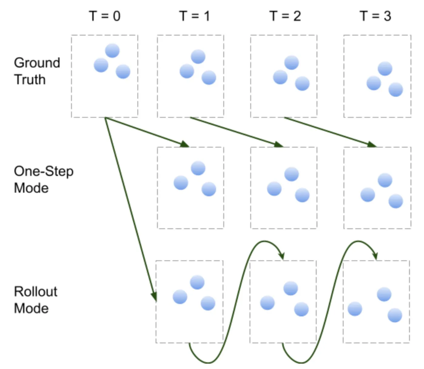
Operation Modes of GNS

The GNS works in two modes: one-step mode and rollout mode. In one-step mode, the GNS always makes predictions with ground-truth inputs. In rollout mode, the GNS predicts positions of particles in the next step based on its own predictions in the previous step. As a result, errors accumulate over time for rollout mode.

One Step Dataset

Each datapoint in this dataset contains trajectories sliced to short time windows. We will use this dataset in the training phase because the history of particles’ states are necessary for the model to make predictions. But in the meantime, since long-horizon prediction is usually inaccurate and time-consuming, we sliced the trajectories to short time windows to improve the perfomance of the model.

class OneStepDataset(pyg.data.Dataset):
    def __init__(self, data_path, split, window_length=7, noise_std=0.0, return_pos=False):
        super().__init__()

        # load dataset from the disk
        with open(os.path.join(data_path, "metadata.json")) as f:
            self.metadata = json.load(f)
        with open(os.path.join(data_path, f"{split}_offset.json")) as f:
            self.offset = json.load(f)
        self.offset = {int(k): v for k, v in self.offset.items()}
        self.window_length = window_length
        self.noise_std = noise_std
        self.return_pos = return_pos

        self.particle_type = np.memmap(os.path.join(data_path, f"{split}_particle_type.dat"), dtype=np.int64, mode="r")
        self.position = np.memmap(os.path.join(data_path, f"{split}_position.dat"), dtype=np.float32, mode="r")

        for traj in self.offset.values():
            self.dim = traj["position"]["shape"][2]
            break

        # cut particle trajectories according to time slices
        self.windows = []
        for traj in self.offset.values():
            size = traj["position"]["shape"][1]
            length = traj["position"]["shape"][0] - window_length + 1
            for i in range(length):
                desc = {
                    "size": size,
                    "type": traj["particle_type"]["offset"],
                    "pos": traj["position"]["offset"] + i * size * self.dim,
                }
                self.windows.append(desc)

    def len(self):
        return len(self.windows)

    def get(self, idx):
        # load corresponding data for this time slice
        window = self.windows[idx]
        size = window["size"]
        particle_type = self.particle_type[window["type"]: window["type"] + size].copy()
        particle_type = torch.from_numpy(particle_type)
        position_seq = self.position[window["pos"]: window["pos"] + self.window_length * size * self.dim].copy()
        position_seq.resize(self.window_length, size, self.dim)
        position_seq = position_seq.transpose(1, 0, 2)
        target_position = position_seq[:, -1]
        position_seq = position_seq[:, :-1]
        target_position = torch.from_numpy(target_position)
        position_seq = torch.from_numpy(position_seq)

        # construct the graph
        with torch.no_grad():
            graph = preprocess(particle_type, position_seq, target_position, self.metadata, self.noise_std)
        if self.return_pos:
          return graph, position_seq[:, -1]
        return graph

Rollout Dataset

Each datapoint in this dataset contains trajectories of particles over 1000 time frames. This dataset is used in the evaluation phase to measure the model’s ability to makie long-horizon predictions.

class RolloutDataset(pyg.data.Dataset):
    def __init__(self, data_path, split, window_length=7):
        super().__init__()

        # load data from the disk
        with open(os.path.join(data_path, "metadata.json")) as f:
            self.metadata = json.load(f)
        with open(os.path.join(data_path, f"{split}_offset.json")) as f:
            self.offset = json.load(f)
        self.offset = {int(k): v for k, v in self.offset.items()}
        self.window_length = window_length

        self.particle_type = np.memmap(os.path.join(data_path, f"{split}_particle_type.dat"), dtype=np.int64, mode="r")
        self.position = np.memmap(os.path.join(data_path, f"{split}_position.dat"), dtype=np.float32, mode="r")

        for traj in self.offset.values():
            self.dim = traj["position"]["shape"][2]
            break

    def len(self):
        return len(self.offset)

    def get(self, idx):
        traj = self.offset[idx]
        size = traj["position"]["shape"][1]
        time_step = traj["position"]["shape"][0]
        particle_type = self.particle_type[traj["particle_type"]["offset"]: traj["particle_type"]["offset"] + size].copy()
        particle_type = torch.from_numpy(particle_type)
        position = self.position[traj["position"]["offset"]: traj["position"]["offset"] + time_step * size * self.dim].copy()
        position.resize(traj["position"]["shape"])
        position = torch.from_numpy(position)
        data = {"particle_type": particle_type, "position": position}
        return data

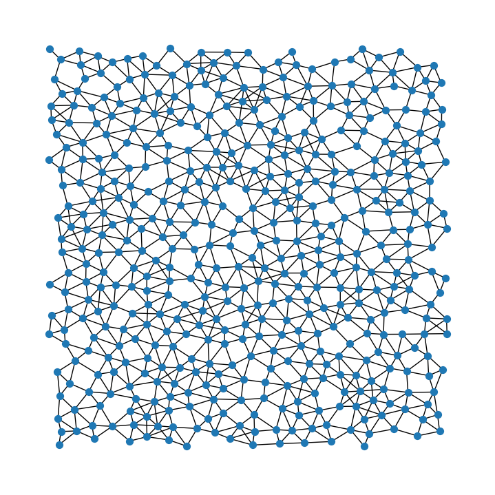
Visualize a graph in the dataset

Each data point in the dataset is a pyg.data.Data object which describes a graph. We explain the contents of the first data point, and visualize the graph.

%matplotlib inline
import matplotlib.pyplot as plt
import networkx as nx

dataset_sample = OneStepDataset(OUTPUT_DIR, "valid", return_pos=True)
graph, position = dataset_sample[0]

print(f"The first item in the valid set is a graph: {graph}")
print(f"This graph has {graph.num_nodes} nodes and {graph.num_edges} edges.")
print(f"Each node is a particle and each edge is the interaction between two particles.")
print(f"Each node has {graph.num_node_features} categorial feature (Data.x), which represents the type of the node.")
print(f"Each node has a {graph.pos.size(1)}-dim feature vector (Data.pos), which represents the positions and velocities of the particle (node) in several frames.")
print(f"Each edge has a {graph.num_edge_features}-dim feature vector (Data.edge_attr), which represents the relative distance and displacement between particles.")
print(f"The model is expected to predict a {graph.y.size(1)}-dim vector for each node (Data.y), which represents the acceleration of the particle.")

# remove directions of edges, because it is a symmetric directed graph.
nx_graph = pyg.utils.to_networkx(graph).to_undirected()
# remove self loops, because every node has a self loop.
nx_graph.remove_edges_from(nx.selfloop_edges(nx_graph))
plt.figure(figsize=(7, 7))
nx.draw(nx_graph, pos={i: tuple(v) for i, v in enumerate(position)}, node_size=50)
plt.show()

The first item in the valid set is a graph: Data(x=[482], edge_index=[2, 3070], edge_attr=[3070, 3], y=[482, 2], pos=[482, 14])
This graph has 482 nodes and 3070 edges.
Each node is a particle and each edge is the interaction between two particles.
Each node has 1 categorial feature (Data.x), which represents the type of the node.
Each node has a 14-dim feature vector (Data.pos), which represents the positions and velocities of the particle (node) in several frames.
Each edge has a 3-dim feature vector (Data.edge_attr), which represents the relative distance and displacement between particles.
The model is expected to predict a 2-dim vector for each node (Data.y), which represents the acceleration of the particle.

GNN Model

We will walk through the implementation of the GNN model in this section!

Helper class

We first define a class for Multi-Layer Perceptron (MLP). This class generates an MLP given the width and the depth of it. Because MLPs are used in several places of the GNN, this helper class will make the code cleaner.

import math
import torch_scatter

class MLP(torch.nn.Module):
    """Multi-Layer perceptron"""
    def __init__(self, input_size, hidden_size, output_size, layers, layernorm=True):
        super().__init__()
        self.layers = torch.nn.ModuleList()
        for i in range(layers):
            self.layers.append(torch.nn.Linear(
                input_size if i == 0 else hidden_size,
                output_size if i == layers - 1 else hidden_size,
            ))
            if i != layers - 1:
                self.layers.append(torch.nn.ReLU())
        if layernorm:
            self.layers.append(torch.nn.LayerNorm(output_size))
        self.reset_parameters()

    def reset_parameters(self):
        for layer in self.layers:
            if isinstance(layer, torch.nn.Linear):
                layer.weight.data.normal_(0, 1 / math.sqrt(layer.in_features))
                layer.bias.data.fill_(0)

    def forward(self, x):
        for layer in self.layers:
            x = layer(x)
        return x

GNN layers

In the following code block, we implement one type of GNN layer named InteractionNetwork (IN), which is proposed by the paper Interaction Networks for Learning about Objects, Relations and Physics.

For a graph \(G\), let the feature of node \(i\) be \(v_i\), and the feature of edge \((i, j)\) be \(e_{i, j}\). There are three stages for IN to generate new features of nodes and edges.

1. Message generation. If there is an edge pointing from node \(i\) to node \(j\), node \(i\) sends a message to node \(j\). The message carries the information of the edge and its two nodes, so it is generated by the following equation \(\mathrm{Msg}_{i,j} = \mathrm{MLP}(v_i, v_j, e_{i,j})\).

2. Message aggregation. In this stage, each node of the graph aggregates all the messages that it received to a fixed-sized representation. In the IN, aggregation means summing all the messages up, i.e., \(\mathrm{Agg}_i=\sum_{(j,i)\in G}\mathrm{Msg}_{i,j}\).

3. Update. Finally, we update features of nodes and edges with the results of previous stages. For each edge, its new feature is simply the sum of its old feature and the correspond message, i.e., \(e'_{i,j}=e_{i,j}+\mathrm{Msg}_{i,j}\). For each node, the new feature is determined by its old feature and the aggregated message, i.e., \(v'_i=v_i+\mathrm{MLP}(v_i, \mathrm{Agg}_i)\).

In PyG, GNN layers are implemented as subclass of MessagePassing. We need to override three critical functions to implement our InteractionNetwork GNN layer. Each function corresponds to one stage of the GNN layer.

1. message() -> message generation

This function controls how a message is generated on each edge of the graph. It takes three arguments: (1) x_i, features of the source nodes; (2) x_j, features of the target nodes; and (3) edge_feature, features of the edges themselves. In the IN, we simply concatenate all these features and generate the messages with an MLP.

1. aggregate() -> message aggregation

This function aggregates messages for nodes. It depends on two arguments: (1) inputs, messages; and (2) index, the graph structure. We handle over the task of message aggregation to the function torch_scatter.scatter and specifies in the argument reduce that we want to sum messages up. Because we want to retain messages themselves to update edge features, we return both messages and aggregated messages.

1. forward() -> update

This function puts everything together. x is the node features, edge_index is the graph structure and edge_feature is edge features. The functionMessagePassing.propagate invokes functions message and aggregate for us. Then, we update node features and edge features and return them.

class InteractionNetwork(pyg.nn.MessagePassing):
    """Interaction Network as proposed in this paper:
    https://proceedings.neurips.cc/paper/2016/hash/3147da8ab4a0437c15ef51a5cc7f2dc4-Abstract.html"""
    def __init__(self, hidden_size, layers):
        super().__init__()
        self.lin_edge = MLP(hidden_size * 3, hidden_size, hidden_size, layers)
        self.lin_node = MLP(hidden_size * 2, hidden_size, hidden_size, layers)

    def forward(self, x, edge_index, edge_feature):
        edge_out, aggr = self.propagate(edge_index, x=(x, x), edge_feature=edge_feature)
        node_out = self.lin_node(torch.cat((x, aggr), dim=-1))
        edge_out = edge_feature + edge_out
        node_out = x + node_out
        return node_out, edge_out

    def message(self, x_i, x_j, edge_feature):
        x = torch.cat((x_i, x_j, edge_feature), dim=-1)
        x = self.lin_edge(x)
        return x

    def aggregate(self, inputs, index, dim_size=None):
        out = torch_scatter.scatter(inputs, index, dim=self.node_dim, dim_size=dim_size, reduce="sum")
        return (inputs, out)

The GNN

Now its time to stack GNN layers to a GNN. Besides GNN layers, there are pre-processing and post-processing blocks in the GNN. Before GNN layers, input features are transformed by MLP so that the expressiveness of GNN is improved without increasing GNN layers. After GNN layers, final outputs (accelerations of particles in our case) are extracted from features generated by GNN layers to meet the requirement of the task.

class LearnedSimulator(torch.nn.Module):
    """Graph Network-based Simulators(GNS)"""
    def __init__(
        self,
        hidden_size=128,
        n_mp_layers=10, # number of GNN layers
        num_particle_types=9,
        particle_type_dim=16, # embedding dimension of particle types
        dim=2, # dimension of the world, typical 2D or 3D
        window_size=5, # the model looks into W frames before the frame to be predicted
    ):
        super().__init__()
        self.window_size = window_size
        self.embed_type = torch.nn.Embedding(num_particle_types, particle_type_dim)
        self.node_in = MLP(particle_type_dim + dim * (window_size + 2), hidden_size, hidden_size, 3)
        self.edge_in = MLP(dim + 1, hidden_size, hidden_size, 3)
        self.node_out = MLP(hidden_size, hidden_size, dim, 3, layernorm=False)
        self.n_mp_layers = n_mp_layers
        self.layers = torch.nn.ModuleList([InteractionNetwork(
            hidden_size, 3
        ) for _ in range(n_mp_layers)])

        self.reset_parameters()

    def reset_parameters(self):
        torch.nn.init.xavier_uniform_(self.embed_type.weight)

    def forward(self, data):
        # pre-processing
        # node feature: combine categorial feature data.x and contiguous feature data.pos.
        node_feature = torch.cat((self.embed_type(data.x), data.pos), dim=-1)
        node_feature = self.node_in(node_feature)
        edge_feature = self.edge_in(data.edge_attr)
        # stack of GNN layers
        for i in range(self.n_mp_layers):
            node_feature, edge_feature = self.layers[i](node_feature, data.edge_index, edge_feature=edge_feature)
        # post-processing
        out = self.node_out(node_feature)
        return out

Training

Before we start training the model, let’s configure the hyperparameters! Since the accessible computaion power is limited in Colab, we will only run 1 epoch of training, which takes about 1.5 hour. Consequently, we won’t be able to produce as accurate results as shown in the original paper in this Colab. Alternatively, we provide a checkpoint of training the model on the entire WaterDrop dataset for 5 epochs, which takes about 14 hours with a GeForce RTX 3080 Ti.

data_path = OUTPUT_DIR
model_path = os.path.join("temp", "models", DATASET_NAME)
rollout_path = os.path.join("temp", "rollouts", DATASET_NAME)

!mkdir -p "$model_path"
!mkdir -p "$rollout_path"

params = {
    "epoch": 1,
    "batch_size": 4,
    "lr": 1e-4,
    "noise": 3e-4,
    "save_interval": 1000,
    "eval_interval": 1000,
    "rollout_interval": 200000,
}

Below are some helper functions for evaluation.

def rollout(model, data, metadata, noise_std):
    device = next(model.parameters()).device
    model.eval()
    window_size = model.window_size + 1
    total_time = data["position"].size(0)
    traj = data["position"][:window_size]
    traj = traj.permute(1, 0, 2)
    particle_type = data["particle_type"]

    for time in range(total_time - window_size):
        with torch.no_grad():
            graph = preprocess(particle_type, traj[:, -window_size:], None, metadata, 0.0)
            graph = graph.to(device)
            acceleration = model(graph).cpu()
            acceleration = acceleration * torch.sqrt(torch.tensor(metadata["acc_std"]) ** 2 + noise_std ** 2) + torch.tensor(metadata["acc_mean"])

            recent_position = traj[:, -1]
            recent_velocity = recent_position - traj[:, -2]
            new_velocity = recent_velocity + acceleration
            new_position = recent_position + new_velocity
            traj = torch.cat((traj, new_position.unsqueeze(1)), dim=1)

    return traj


def oneStepMSE(simulator, dataloader, metadata, noise):
    """Returns two values, loss and MSE"""
    total_loss = 0.0
    total_mse = 0.0
    batch_count = 0
    simulator.eval()
    with torch.no_grad():
        scale = torch.sqrt(torch.tensor(metadata["acc_std"]) ** 2 + noise ** 2).cuda()
        for data in valid_loader:
            data = data.cuda()
            pred = simulator(data)
            mse = ((pred - data.y) * scale) ** 2
            mse = mse.sum(dim=-1).mean()
            loss = ((pred - data.y) ** 2).mean()
            total_mse += mse.item()
            total_loss += loss.item()
            batch_count += 1
    return total_loss / batch_count, total_mse / batch_count


def rolloutMSE(simulator, dataset, noise):
    total_loss = 0.0
    batch_count = 0
    simulator.eval()
    with torch.no_grad():
        for rollout_data in dataset:
            rollout_out = rollout(simulator, rollout_data, dataset.metadata, noise)
            rollout_out = rollout_out.permute(1, 0, 2)
            loss = (rollout_out - rollout_data["position"]) ** 2
            loss = loss.sum(dim=-1).mean()
            total_loss += loss.item()
            batch_count += 1
    return total_loss / batch_count

Here is the main training loop!

from tqdm import tqdm

def train(params, simulator, train_loader, valid_loader, valid_rollout_dataset):
    loss_fn = torch.nn.MSELoss()
    optimizer = torch.optim.Adam(simulator.parameters(), lr=params["lr"])
    scheduler = torch.optim.lr_scheduler.ExponentialLR(optimizer, gamma=0.1 ** (1 / 5e6))

    # recording loss curve
    train_loss_list = []
    eval_loss_list = []
    onestep_mse_list = []
    rollout_mse_list = []
    total_step = 0

    for i in range(params["epoch"]):
        simulator.train()
        progress_bar = tqdm(train_loader, desc=f"Epoch {i}")
        total_loss = 0
        batch_count = 0
        for data in progress_bar:
            optimizer.zero_grad()
            data = data.cuda()
            pred = simulator(data)
            loss = loss_fn(pred, data.y)
            loss.backward()
            optimizer.step()
            scheduler.step()
            total_loss += loss.item()
            batch_count += 1
            progress_bar.set_postfix({"loss": loss.item(), "avg_loss": total_loss / batch_count, "lr": optimizer.param_groups[0]["lr"]})
            total_step += 1
            train_loss_list.append((total_step, loss.item()))

            # evaluation
            if total_step % params["eval_interval"] == 0:
                simulator.eval()
                eval_loss, onestep_mse = oneStepMSE(simulator, valid_loader, valid_dataset.metadata, params["noise"])
                eval_loss_list.append((total_step, eval_loss))
                onestep_mse_list.append((total_step, onestep_mse))
                tqdm.write(f"\nEval: Loss: {eval_loss}, One Step MSE: {onestep_mse}")
                simulator.train()

            # do rollout on valid set
            if total_step % params["rollout_interval"] == 0:
                simulator.eval()
                rollout_mse = rolloutMSE(simulator, valid_rollout_dataset, params["noise"])
                rollout_mse_list.append((total_step, rollout_mse))
                tqdm.write(f"\nEval: Rollout MSE: {rollout_mse}")
                simulator.train()

            # save model
            if total_step % params["save_interval"] == 0:
                torch.save(
                    {
                        "model": simulator.state_dict(),
                        "optimizer": optimizer.state_dict(),
                        "scheduler": scheduler.state_dict(),
                    },
                    os.path.join(model_path, f"checkpoint_{total_step}.pt")
                )
    return train_loss_list, eval_loss_list, onestep_mse_list, rollout_mse_list

Finally, let’s load the dataset and train the model! It takes roughly 1.5 hour to run this block on Colab with the default parameters. If you are impatient, we highly recommend you to skip the next 2 blocks and load the checkpoint we provided to save some time; otherwise, make a cup of tea/coffee and come back later to see the results of training!

# Training the model is time-consuming. We highly recommend you to skip this block and load the checkpoint in the next block.

# load dataset
train_dataset = OneStepDataset(data_path, "train", noise_std=params["noise"])
valid_dataset = OneStepDataset(data_path, "valid", noise_std=params["noise"])
train_loader = pyg.loader.DataLoader(train_dataset, batch_size=params["batch_size"], shuffle=True, pin_memory=True, num_workers=2)
valid_loader = pyg.loader.DataLoader(valid_dataset, batch_size=params["batch_size"], shuffle=False, pin_memory=True, num_workers=2)
valid_rollout_dataset = RolloutDataset(data_path, "valid")

# build model
simulator = LearnedSimulator()
simulator = simulator.cuda()

# train the model
train_loss_list, eval_loss_list, onestep_mse_list, rollout_mse_list = train(params, simulator, train_loader, valid_loader, valid_rollout_dataset)

Epoch 0: 100%|██████████| 249/249 [00:18<00:00, 13.20it/s, loss=0.99, avg_loss=1.06, lr=0.0001]
Epoch 1: 100%|██████████| 249/249 [00:19<00:00, 12.80it/s, loss=0.944, avg_loss=1.03, lr=0.0001]
Epoch 2: 100%|██████████| 249/249 [00:18<00:00, 13.13it/s, loss=0.919, avg_loss=1.02, lr=0.0001]
Epoch 3: 100%|██████████| 249/249 [00:19<00:00, 12.97it/s, loss=1.09, avg_loss=1.03, lr=0.0001]
Epoch 4:   1%|          | 3/249 [00:06<00:24, 10.14it/s, loss=0.984, avg_loss=1.25, lr=0.0001]

Eval: Loss: 0.9624428978885513, One Step MSE: 1.8485395512918302e-07

Epoch 4: 100%|██████████| 249/249 [00:25<00:00,  9.75it/s, loss=1.46, avg_loss=1.02, lr=9.99e-5]
Epoch 5: 100%|██████████| 249/249 [00:19<00:00, 13.08it/s, loss=0.927, avg_loss=1.02, lr=9.99e-5]
Epoch 6: 100%|██████████| 249/249 [00:18<00:00, 13.14it/s, loss=0.953, avg_loss=1.02, lr=9.99e-5]
Epoch 7: 100%|██████████| 249/249 [00:19<00:00, 13.05it/s, loss=0.882, avg_loss=1.01, lr=9.99e-5]
Epoch 8:   3%|▎         | 7/249 [00:07<00:20, 11.94it/s, loss=0.929, avg_loss=0.952, lr=9.99e-5]

Eval: Loss: 0.9490157880457529, One Step MSE: 1.8224882540902668e-07

Epoch 8: 100%|██████████| 249/249 [00:26<00:00,  9.56it/s, loss=1.02, avg_loss=1.01, lr=9.99e-5]
Epoch 9: 100%|██████████| 249/249 [00:18<00:00, 13.23it/s, loss=0.688, avg_loss=0.849, lr=9.99e-5]
Epoch 10: 100%|██████████| 249/249 [00:19<00:00, 13.00it/s, loss=0.642, avg_loss=0.623, lr=9.99e-5]
Epoch 11: 100%|██████████| 249/249 [00:18<00:00, 13.20it/s, loss=0.243, avg_loss=0.45, lr=9.99e-5]
Epoch 12:   5%|▌         | 13/249 [00:08<05:16,  1.34s/it, loss=0.326, avg_loss=0.377, lr=9.99e-5]

Eval: Loss: 0.38679184983054316, One Step MSE: 7.41684273230222e-08

Epoch 12: 100%|██████████| 249/249 [00:26<00:00,  9.40it/s, loss=0.507, avg_loss=0.38, lr=9.99e-5]
Epoch 13: 100%|██████████| 249/249 [00:19<00:00, 13.09it/s, loss=0.216, avg_loss=0.372, lr=9.98e-5]
Epoch 14: 100%|██████████| 249/249 [00:19<00:00, 13.03it/s, loss=0.174, avg_loss=0.32, lr=9.98e-5]
Epoch 15: 100%|██████████| 249/249 [00:18<00:00, 13.21it/s, loss=0.283, avg_loss=0.302, lr=9.98e-5]
Epoch 16:   7%|▋         | 17/249 [00:08<04:39,  1.21s/it, loss=0.308, avg_loss=0.327, lr=9.98e-5]

Eval: Loss: 0.27295780002352704, One Step MSE: 5.234293432779514e-08

Epoch 16: 100%|██████████| 249/249 [00:26<00:00,  9.55it/s, loss=0.792, avg_loss=0.288, lr=9.98e-5]
Epoch 17: 100%|██████████| 249/249 [00:19<00:00, 12.98it/s, loss=0.291, avg_loss=0.277, lr=9.98e-5]
Epoch 18: 100%|██████████| 249/249 [00:18<00:00, 13.22it/s, loss=0.16, avg_loss=0.27, lr=9.98e-5]
Epoch 19: 100%|██████████| 249/249 [00:19<00:00, 13.03it/s, loss=0.362, avg_loss=0.258, lr=9.98e-5]
Epoch 20:   8%|▊         | 21/249 [00:08<04:01,  1.06s/it, loss=0.175, avg_loss=0.297, lr=9.98e-5]

Eval: Loss: 0.21626010130208181, One Step MSE: 4.1469931403183634e-08

Epoch 20: 100%|██████████| 249/249 [00:25<00:00,  9.80it/s, loss=0.475, avg_loss=0.545, lr=9.98e-5]
Epoch 21: 100%|██████████| 249/249 [00:18<00:00, 13.18it/s, loss=0.139, avg_loss=0.322, lr=9.97e-5]
Epoch 22: 100%|██████████| 249/249 [00:18<00:00, 13.26it/s, loss=0.274, avg_loss=0.273, lr=9.97e-5]
Epoch 23: 100%|██████████| 249/249 [00:19<00:00, 13.02it/s, loss=0.278, avg_loss=0.259, lr=9.97e-5]
Epoch 24:  10%|█         | 25/249 [00:09<04:22,  1.17s/it, loss=0.212, avg_loss=0.256, lr=9.97e-5]

Eval: Loss: 0.2310676653701139, One Step MSE: 4.4428789914355e-08

Epoch 24: 100%|██████████| 249/249 [00:26<00:00,  9.50it/s, loss=0.188, avg_loss=0.248, lr=9.97e-5]
Epoch 25: 100%|██████████| 249/249 [00:18<00:00, 13.17it/s, loss=0.532, avg_loss=0.245, lr=9.97e-5]
Epoch 26: 100%|██████████| 249/249 [00:19<00:00, 13.00it/s, loss=0.213, avg_loss=0.24, lr=9.97e-5]
Epoch 27: 100%|██████████| 249/249 [00:18<00:00, 13.14it/s, loss=0.163, avg_loss=0.222, lr=9.97e-5]
Epoch 28:  12%|█▏        | 29/249 [00:08<03:46,  1.03s/it, loss=0.147, avg_loss=0.312, lr=9.97e-5]

Eval: Loss: 0.20556915662135464, One Step MSE: 3.9413650388912933e-08

Epoch 28: 100%|██████████| 249/249 [00:25<00:00,  9.70it/s, loss=0.187, avg_loss=0.228, lr=9.97e-5]
Epoch 29: 100%|██████████| 249/249 [00:18<00:00, 13.13it/s, loss=0.233, avg_loss=0.257, lr=9.97e-5]
Epoch 30: 100%|██████████| 249/249 [00:19<00:00, 12.91it/s, loss=0.119, avg_loss=0.221, lr=9.96e-5]
Epoch 31: 100%|██████████| 249/249 [00:18<00:00, 13.16it/s, loss=0.172, avg_loss=0.216, lr=9.96e-5]
Epoch 32:  13%|█▎        | 33/249 [00:09<04:09,  1.15s/it, loss=0.175, avg_loss=0.18, lr=9.96e-5]

Eval: Loss: 0.17550723544924135, One Step MSE: 3.365333827941347e-08

Epoch 32: 100%|██████████| 249/249 [00:26<00:00,  9.54it/s, loss=0.124, avg_loss=0.208, lr=9.96e-5]
Epoch 33: 100%|██████████| 249/249 [00:19<00:00, 12.97it/s, loss=0.155, avg_loss=0.2, lr=9.96e-5]
Epoch 34: 100%|██████████| 249/249 [00:18<00:00, 13.18it/s, loss=0.182, avg_loss=0.218, lr=9.96e-5]
Epoch 35: 100%|██████████| 249/249 [00:19<00:00, 12.98it/s, loss=0.207, avg_loss=0.206, lr=9.96e-5]
Epoch 36:  14%|█▍        | 35/249 [00:09<00:15, 13.85it/s, loss=0.2, avg_loss=0.194, lr=9.96e-5]

Eval: Loss: 0.1836872404239264, One Step MSE: 3.5251602233439464e-08

Epoch 36: 100%|██████████| 249/249 [00:25<00:00,  9.60it/s, loss=0.139, avg_loss=0.21, lr=9.96e-5]
Epoch 37: 100%|██████████| 249/249 [00:18<00:00, 13.11it/s, loss=0.147, avg_loss=0.196, lr=9.96e-5]
Epoch 38: 100%|██████████| 249/249 [00:19<00:00, 12.97it/s, loss=0.189, avg_loss=0.195, lr=9.96e-5]
Epoch 39: 100%|██████████| 249/249 [00:18<00:00, 13.15it/s, loss=1.2, avg_loss=0.19, lr=9.95e-5]
Epoch 40:  16%|█▋        | 41/249 [00:09<03:35,  1.04s/it, loss=0.204, avg_loss=0.255, lr=9.95e-5]

Eval: Loss: 0.19442890309186345, One Step MSE: 3.729126256875833e-08

Epoch 40: 100%|██████████| 249/249 [00:25<00:00,  9.66it/s, loss=0.152, avg_loss=0.203, lr=9.95e-5]
Epoch 41: 100%|██████████| 249/249 [00:19<00:00, 13.05it/s, loss=0.11, avg_loss=0.196, lr=9.95e-5]
Epoch 42: 100%|██████████| 249/249 [00:19<00:00, 13.02it/s, loss=0.106, avg_loss=0.176, lr=9.95e-5]
Epoch 43: 100%|██████████| 249/249 [00:19<00:00, 13.03it/s, loss=0.212, avg_loss=0.178, lr=9.95e-5]
Epoch 44:  18%|█▊        | 45/249 [00:10<03:52,  1.14s/it, loss=0.1, avg_loss=0.154, lr=9.95e-5]

Eval: Loss: 0.15783582373436197, One Step MSE: 3.032950739463374e-08

Epoch 44: 100%|██████████| 249/249 [00:26<00:00,  9.57it/s, loss=0.0784, avg_loss=0.17, lr=9.95e-5]
Epoch 45: 100%|██████████| 249/249 [00:19<00:00, 13.02it/s, loss=0.0987, avg_loss=0.198, lr=9.95e-5]
Epoch 46: 100%|██████████| 249/249 [00:18<00:00, 13.14it/s, loss=0.0961, avg_loss=0.161, lr=9.95e-5]
Epoch 47: 100%|██████████| 249/249 [00:19<00:00, 12.98it/s, loss=0.135, avg_loss=0.195, lr=9.95e-5]
Epoch 48:  20%|█▉        | 49/249 [00:10<03:49,  1.15s/it, loss=0.123, avg_loss=0.142, lr=9.94e-5]

Eval: Loss: 0.13785184548801208, One Step MSE: 2.645640632942192e-08

Epoch 48: 100%|██████████| 249/249 [00:26<00:00,  9.51it/s, loss=0.131, avg_loss=0.164, lr=9.94e-5]
Epoch 49: 100%|██████████| 249/249 [00:18<00:00, 13.16it/s, loss=0.131, avg_loss=0.166, lr=9.94e-5]
Epoch 50: 100%|██████████| 249/249 [00:19<00:00, 12.98it/s, loss=0.597, avg_loss=0.166, lr=9.94e-5]
Epoch 51: 100%|██████████| 249/249 [00:18<00:00, 13.16it/s, loss=0.129, avg_loss=0.164, lr=9.94e-5]
Epoch 52:  21%|██▏       | 53/249 [00:10<03:18,  1.01s/it, loss=0.188, avg_loss=0.133, lr=9.94e-5]

Eval: Loss: 0.12809966244252333, One Step MSE: 2.457434036360732e-08

Epoch 52: 100%|██████████| 249/249 [00:25<00:00,  9.77it/s, loss=0.14, avg_loss=0.163, lr=9.94e-5]
Epoch 53: 100%|██████████| 249/249 [00:19<00:00, 13.00it/s, loss=0.532, avg_loss=0.167, lr=9.94e-5]
Epoch 54: 100%|██████████| 249/249 [00:19<00:00, 13.03it/s, loss=0.0955, avg_loss=0.161, lr=9.94e-5]
Epoch 55: 100%|██████████| 249/249 [00:19<00:00, 13.04it/s, loss=0.161, avg_loss=0.155, lr=9.94e-5]
Epoch 56:  23%|██▎       | 57/249 [00:11<03:37,  1.13s/it, loss=0.134, avg_loss=0.176, lr=9.94e-5]

Eval: Loss: 0.14424636520176048, One Step MSE: 2.7674898071554718e-08

Epoch 56: 100%|██████████| 249/249 [00:25<00:00,  9.58it/s, loss=0.0919, avg_loss=0.156, lr=9.93e-5]
Epoch 57: 100%|██████████| 249/249 [00:19<00:00, 12.93it/s, loss=0.15, avg_loss=0.166, lr=9.93e-5]
Epoch 58: 100%|██████████| 249/249 [00:19<00:00, 13.10it/s, loss=0.127, avg_loss=0.15, lr=9.93e-5]
Epoch 59: 100%|██████████| 249/249 [00:19<00:00, 12.87it/s, loss=0.125, avg_loss=0.164, lr=9.93e-5]
Epoch 60:  24%|██▍       | 61/249 [00:11<03:36,  1.15s/it, loss=0.104, avg_loss=0.142, lr=9.93e-5]

Eval: Loss: 0.14786650476805177, One Step MSE: 2.8390447094533597e-08

Epoch 60: 100%|██████████| 249/249 [00:26<00:00,  9.52it/s, loss=0.0705, avg_loss=0.183, lr=9.93e-5]
Epoch 61: 100%|██████████| 249/249 [00:18<00:00, 13.19it/s, loss=0.115, avg_loss=0.147, lr=9.93e-5]
Epoch 62: 100%|██████████| 249/249 [00:19<00:00, 12.89it/s, loss=0.0938, avg_loss=0.148, lr=9.93e-5]
Epoch 63: 100%|██████████| 249/249 [00:18<00:00, 13.18it/s, loss=0.094, avg_loss=0.151, lr=9.93e-5]
Epoch 64:  26%|██▌       | 65/249 [00:11<03:06,  1.01s/it, loss=0.119, avg_loss=0.15, lr=9.93e-5]

Eval: Loss: 0.14944408450978827, One Step MSE: 2.871252687460431e-08

Epoch 64: 100%|██████████| 249/249 [00:25<00:00,  9.81it/s, loss=0.161, avg_loss=0.144, lr=9.93e-5]
Epoch 65: 100%|██████████| 249/249 [00:19<00:00, 13.04it/s, loss=0.174, avg_loss=0.14, lr=9.92e-5]
Epoch 66: 100%|██████████| 249/249 [00:18<00:00, 13.14it/s, loss=0.117, avg_loss=0.139, lr=9.92e-5]
Epoch 67: 100%|██████████| 249/249 [00:19<00:00, 12.92it/s, loss=0.143, avg_loss=0.135, lr=9.92e-5]
Epoch 68:  28%|██▊       | 69/249 [00:12<03:23,  1.13s/it, loss=0.566, avg_loss=0.711, lr=9.92e-5]

Eval: Loss: 0.6050984430983364, One Step MSE: 1.1683671815663513e-07

Epoch 68: 100%|██████████| 249/249 [00:25<00:00,  9.59it/s, loss=0.148, avg_loss=0.502, lr=9.92e-5]
Epoch 69: 100%|██████████| 249/249 [00:19<00:00, 13.09it/s, loss=0.17, avg_loss=0.253, lr=9.92e-5]
Epoch 70: 100%|██████████| 249/249 [00:18<00:00, 13.14it/s, loss=0.454, avg_loss=0.21, lr=9.92e-5]
Epoch 71: 100%|██████████| 249/249 [00:19<00:00, 12.99it/s, loss=0.127, avg_loss=0.203, lr=9.92e-5]
Epoch 72:  29%|██▉       | 73/249 [00:12<03:24,  1.16s/it, loss=0.113, avg_loss=0.168, lr=9.92e-5]

Eval: Loss: 0.144893929182765, One Step MSE: 2.7817969746543924e-08

Epoch 72: 100%|██████████| 249/249 [00:26<00:00,  9.55it/s, loss=0.192, avg_loss=0.191, lr=9.92e-5]
Epoch 73: 100%|██████████| 249/249 [00:18<00:00, 13.16it/s, loss=0.141, avg_loss=0.183, lr=9.92e-5]
Epoch 74: 100%|██████████| 249/249 [00:19<00:00, 13.02it/s, loss=0.128, avg_loss=0.189, lr=9.91e-5]
Epoch 75: 100%|██████████| 249/249 [00:18<00:00, 13.13it/s, loss=0.379, avg_loss=0.151, lr=9.91e-5]
Epoch 76:  31%|███       | 77/249 [00:12<02:52,  1.00s/it, loss=0.169, avg_loss=0.147, lr=9.91e-5]

Eval: Loss: 0.14855602290855355, One Step MSE: 2.850924411494721e-08

Epoch 76: 100%|██████████| 249/249 [00:25<00:00,  9.82it/s, loss=0.144, avg_loss=0.168, lr=9.91e-5]
Epoch 77: 100%|██████████| 249/249 [00:19<00:00, 13.00it/s, loss=0.165, avg_loss=0.16, lr=9.91e-5]
Epoch 78: 100%|██████████| 249/249 [00:18<00:00, 13.19it/s, loss=0.11, avg_loss=0.145, lr=9.91e-5]
Epoch 79: 100%|██████████| 249/249 [00:19<00:00, 12.96it/s, loss=0.138, avg_loss=0.151, lr=9.91e-5]
Epoch 80:  33%|███▎      | 81/249 [00:13<03:13,  1.15s/it, loss=0.0722, avg_loss=0.129, lr=9.91e-5]

Eval: Loss: 0.12400319343470187, One Step MSE: 2.379293122719236e-08

Epoch 80: 100%|██████████| 249/249 [00:26<00:00,  9.52it/s, loss=0.117, avg_loss=0.143, lr=9.91e-5]
Epoch 81: 100%|██████████| 249/249 [00:18<00:00, 13.23it/s, loss=0.178, avg_loss=0.141, lr=9.91e-5]
Epoch 82: 100%|██████████| 249/249 [00:19<00:00, 13.00it/s, loss=0.142, avg_loss=0.152, lr=9.91e-5]
Epoch 83: 100%|██████████| 249/249 [00:18<00:00, 13.14it/s, loss=0.0937, avg_loss=0.15, lr=9.9e-5]
Epoch 84:  34%|███▍      | 85/249 [00:13<02:51,  1.05s/it, loss=0.162, avg_loss=0.166, lr=9.9e-5]

Eval: Loss: 0.1648225225358603, One Step MSE: 3.160742100891937e-08

Epoch 84: 100%|██████████| 249/249 [00:25<00:00,  9.72it/s, loss=0.0628, avg_loss=0.15, lr=9.9e-5]
Epoch 85: 100%|██████████| 249/249 [00:19<00:00, 13.03it/s, loss=0.101, avg_loss=0.129, lr=9.9e-5]
Epoch 86: 100%|██████████| 249/249 [00:19<00:00, 13.08it/s, loss=0.0984, avg_loss=0.15, lr=9.9e-5]
Epoch 87: 100%|██████████| 249/249 [00:18<00:00, 13.11it/s, loss=0.102, avg_loss=0.147, lr=9.9e-5]
Epoch 88:  36%|███▌      | 89/249 [00:13<02:41,  1.01s/it, loss=0.0964, avg_loss=0.137, lr=9.9e-5]

Eval: Loss: 0.11691469980411262, One Step MSE: 2.2448665462894063e-08

Epoch 88: 100%|██████████| 249/249 [00:25<00:00,  9.87it/s, loss=0.0849, avg_loss=0.133, lr=9.9e-5]
Epoch 89: 100%|██████████| 249/249 [00:19<00:00, 13.03it/s, loss=0.0729, avg_loss=0.128, lr=9.9e-5]
Epoch 90: 100%|██████████| 249/249 [00:18<00:00, 13.16it/s, loss=0.0932, avg_loss=0.123, lr=9.9e-5]
Epoch 91: 100%|██████████| 249/249 [00:19<00:00, 13.03it/s, loss=0.14, avg_loss=0.133, lr=9.9e-5]
Epoch 92:  37%|███▋      | 93/249 [00:14<02:56,  1.13s/it, loss=0.129, avg_loss=0.175, lr=9.89e-5]

Eval: Loss: 0.13324948222223057, One Step MSE: 2.5614396508340213e-08

Epoch 92: 100%|██████████| 249/249 [00:25<00:00,  9.60it/s, loss=0.101, avg_loss=0.146, lr=9.89e-5]
Epoch 93: 100%|██████████| 249/249 [00:18<00:00, 13.19it/s, loss=0.108, avg_loss=0.142, lr=9.89e-5]
Epoch 94: 100%|██████████| 249/249 [00:19<00:00, 12.99it/s, loss=0.0709, avg_loss=0.117, lr=9.89e-5]
Epoch 95: 100%|██████████| 249/249 [00:18<00:00, 13.19it/s, loss=0.169, avg_loss=0.139, lr=9.89e-5]
Epoch 96:  39%|███▉      | 97/249 [00:13<02:30,  1.01it/s, loss=0.11, avg_loss=0.13, lr=9.89e-5]

Eval: Loss: 0.12618800369371852, One Step MSE: 2.4174850794114734e-08

Epoch 96: 100%|██████████| 249/249 [00:25<00:00,  9.87it/s, loss=0.0948, avg_loss=0.125, lr=9.89e-5]
Epoch 97: 100%|██████████| 249/249 [00:19<00:00, 13.09it/s, loss=0.167, avg_loss=0.131, lr=9.89e-5]
Epoch 98: 100%|██████████| 249/249 [00:18<00:00, 13.12it/s, loss=0.0606, avg_loss=0.117, lr=9.89e-5]
Epoch 99: 100%|██████████| 249/249 [00:19<00:00, 12.77it/s, loss=0.0538, avg_loss=0.118, lr=9.89e-5]
Epoch 100:  41%|████      | 101/249 [00:14<02:45,  1.12s/it, loss=0.242, avg_loss=0.0987, lr=9.89e-5]

Eval: Loss: 0.10524629580088887, One Step MSE: 2.018601811540912e-08

Epoch 100: 100%|██████████| 249/249 [00:25<00:00,  9.62it/s, loss=0.094, avg_loss=0.119, lr=9.88e-5]
Epoch 101: 100%|██████████| 249/249 [00:18<00:00, 13.17it/s, loss=0.101, avg_loss=0.113, lr=9.88e-5]
Epoch 102: 100%|██████████| 249/249 [00:19<00:00, 12.97it/s, loss=0.107, avg_loss=0.114, lr=9.88e-5]
Epoch 103: 100%|██████████| 249/249 [00:18<00:00, 13.18it/s, loss=0.33, avg_loss=0.125, lr=9.88e-5]
Epoch 104:  42%|████▏     | 104/249 [00:15<02:47,  1.15s/it, loss=0.103, avg_loss=0.119, lr=9.88e-5]

Eval: Loss: 0.11374883907267368, One Step MSE: 2.182236234464669e-08

Epoch 104: 100%|██████████| 249/249 [00:26<00:00,  9.48it/s, loss=0.057, avg_loss=0.122, lr=9.88e-5]
Epoch 105: 100%|██████████| 249/249 [00:19<00:00, 13.10it/s, loss=0.0677, avg_loss=0.111, lr=9.88e-5]
Epoch 106: 100%|██████████| 249/249 [00:18<00:00, 13.11it/s, loss=0.0666, avg_loss=0.11, lr=9.88e-5]
Epoch 107: 100%|██████████| 249/249 [00:18<00:00, 13.15it/s, loss=0.1, avg_loss=0.112, lr=9.88e-5]
Epoch 108:  44%|████▍     | 109/249 [00:14<02:20,  1.00s/it, loss=0.0576, avg_loss=0.117, lr=9.88e-5]

Eval: Loss: 0.11051016595648475, One Step MSE: 2.120191918149077e-08

Epoch 108: 100%|██████████| 249/249 [00:25<00:00,  9.90it/s, loss=0.0856, avg_loss=0.106, lr=9.88e-5]
Epoch 109: 100%|██████████| 249/249 [00:19<00:00, 13.05it/s, loss=0.115, avg_loss=0.117, lr=9.87e-5]
Epoch 110: 100%|██████████| 249/249 [00:19<00:00, 13.03it/s, loss=0.0569, avg_loss=0.12, lr=9.87e-5]
Epoch 111: 100%|██████████| 249/249 [00:19<00:00, 13.05it/s, loss=0.0798, avg_loss=0.108, lr=9.87e-5]
Epoch 112:  45%|████▌     | 113/249 [00:15<02:34,  1.13s/it, loss=0.223, avg_loss=0.105, lr=9.87e-5]

Eval: Loss: 0.10954236403765927, One Step MSE: 2.102910051715857e-08

Epoch 112: 100%|██████████| 249/249 [00:25<00:00,  9.58it/s, loss=0.111, avg_loss=0.109, lr=9.87e-5]
Epoch 113: 100%|██████████| 249/249 [00:18<00:00, 13.22it/s, loss=0.105, avg_loss=0.113, lr=9.87e-5]
Epoch 114: 100%|██████████| 249/249 [00:19<00:00, 12.96it/s, loss=0.114, avg_loss=0.131, lr=9.87e-5]
Epoch 115: 100%|██████████| 249/249 [00:18<00:00, 13.18it/s, loss=0.0644, avg_loss=0.109, lr=9.87e-5]
Epoch 116:  47%|████▋     | 117/249 [00:15<02:17,  1.04s/it, loss=0.0623, avg_loss=0.0991, lr=9.87e-5]

Eval: Loss: 0.10758851274070012, One Step MSE: 2.063654977201375e-08

Epoch 116: 100%|██████████| 249/249 [00:25<00:00,  9.76it/s, loss=0.0584, avg_loss=0.106, lr=9.87e-5]
Epoch 117: 100%|██████████| 249/249 [00:19<00:00, 13.01it/s, loss=0.144, avg_loss=0.104, lr=9.87e-5]
Epoch 118: 100%|██████████| 249/249 [00:18<00:00, 13.16it/s, loss=0.0652, avg_loss=0.103, lr=9.86e-5]
Epoch 119: 100%|██████████| 249/249 [00:19<00:00, 13.02it/s, loss=0.0772, avg_loss=0.103, lr=9.86e-5]
Epoch 120:  49%|████▊     | 121/249 [00:15<02:10,  1.02s/it, loss=0.0802, avg_loss=0.0972, lr=9.86e-5]

Eval: Loss: 0.10604566729152538, One Step MSE: 2.0336590473204115e-08

Epoch 120: 100%|██████████| 249/249 [00:25<00:00,  9.85it/s, loss=0.115, avg_loss=0.0976, lr=9.86e-5]
Epoch 121: 100%|██████████| 249/249 [00:18<00:00, 13.21it/s, loss=0.075, avg_loss=0.119, lr=9.86e-5]
Epoch 122: 100%|██████████| 249/249 [00:19<00:00, 13.04it/s, loss=0.148, avg_loss=0.106, lr=9.86e-5]
Epoch 123: 100%|██████████| 249/249 [00:18<00:00, 13.20it/s, loss=0.106, avg_loss=0.0996, lr=9.86e-5]
Epoch 124:  50%|█████     | 125/249 [00:16<02:21,  1.14s/it, loss=0.126, avg_loss=0.111, lr=9.86e-5]

Eval: Loss: 0.1566714323668116, One Step MSE: 3.007668484280632e-08

Epoch 124: 100%|██████████| 249/249 [00:26<00:00,  9.57it/s, loss=0.146, avg_loss=0.123, lr=9.86e-5]
Epoch 125: 100%|██████████| 249/249 [00:19<00:00, 13.09it/s, loss=0.0366, avg_loss=0.0992, lr=9.86e-5]
Epoch 126: 100%|██████████| 249/249 [00:19<00:00, 13.09it/s, loss=0.102, avg_loss=0.109, lr=9.86e-5]
Epoch 127: 100%|██████████| 249/249 [00:19<00:00, 13.10it/s, loss=0.0973, avg_loss=0.0968, lr=9.85e-5]
Epoch 128:  52%|█████▏    | 129/249 [00:15<01:57,  1.02it/s, loss=0.0786, avg_loss=0.0855, lr=9.85e-5]

Eval: Loss: 0.10072930170649505, One Step MSE: 1.9310580283410304e-08

Epoch 128: 100%|██████████| 249/249 [00:25<00:00,  9.92it/s, loss=0.133, avg_loss=0.0956, lr=9.85e-5]
Epoch 129: 100%|██████████| 249/249 [00:19<00:00, 13.07it/s, loss=0.051, avg_loss=0.111, lr=9.85e-5]
Epoch 130: 100%|██████████| 249/249 [00:18<00:00, 13.15it/s, loss=0.0417, avg_loss=0.0968, lr=9.85e-5]
Epoch 131: 100%|██████████| 249/249 [00:19<00:00, 13.00it/s, loss=0.0748, avg_loss=0.109, lr=9.85e-5]
Epoch 132:  53%|█████▎    | 133/249 [00:16<02:04,  1.08s/it, loss=0.0772, avg_loss=0.0851, lr=9.85e-5]

Eval: Loss: 0.09611847673554018, One Step MSE: 1.84352522431053e-08

Epoch 132: 100%|██████████| 249/249 [00:25<00:00,  9.74it/s, loss=0.385, avg_loss=0.105, lr=9.85e-5]
Epoch 133: 100%|██████████| 249/249 [00:18<00:00, 13.13it/s, loss=0.0835, avg_loss=0.0995, lr=9.85e-5]
Epoch 134: 100%|██████████| 249/249 [00:19<00:00, 13.06it/s, loss=0.155, avg_loss=0.0936, lr=9.85e-5]
Epoch 135: 100%|██████████| 249/249 [00:18<00:00, 13.20it/s, loss=0.0961, avg_loss=0.0976, lr=9.85e-5]
Epoch 136:  55%|█████▌    | 137/249 [00:17<02:07,  1.14s/it, loss=0.0664, avg_loss=0.098, lr=9.84e-5]

Eval: Loss: 0.09164998303335833, One Step MSE: 1.7595847715068703e-08

Epoch 136: 100%|██████████| 249/249 [00:25<00:00,  9.62it/s, loss=0.0504, avg_loss=0.0959, lr=9.84e-5]
Epoch 137: 100%|██████████| 249/249 [00:18<00:00, 13.12it/s, loss=0.0804, avg_loss=0.0905, lr=9.84e-5]
Epoch 138: 100%|██████████| 249/249 [00:18<00:00, 13.25it/s, loss=0.0366, avg_loss=0.091, lr=9.84e-5]
Epoch 139: 100%|██████████| 249/249 [00:19<00:00, 13.01it/s, loss=0.0664, avg_loss=0.0933, lr=9.84e-5]
Epoch 140:  57%|█████▋    | 141/249 [00:16<01:46,  1.02it/s, loss=0.0627, avg_loss=0.0961, lr=9.84e-5]

Eval: Loss: 0.09332117309651701, One Step MSE: 1.7892347111277412e-08

Epoch 140: 100%|██████████| 249/249 [00:25<00:00,  9.87it/s, loss=0.0443, avg_loss=0.0913, lr=9.84e-5]
Epoch 141: 100%|██████████| 249/249 [00:18<00:00, 13.20it/s, loss=0.101, avg_loss=0.0951, lr=9.84e-5]
Epoch 142: 100%|██████████| 249/249 [00:19<00:00, 13.07it/s, loss=0.105, avg_loss=0.0929, lr=9.84e-5]
Epoch 143: 100%|██████████| 249/249 [00:18<00:00, 13.19it/s, loss=0.108, avg_loss=0.0973, lr=9.84e-5]
Epoch 144:  58%|█████▊    | 145/249 [00:18<01:57,  1.13s/it, loss=0.0908, avg_loss=0.0951, lr=9.84e-5]

Eval: Loss: 0.11163777726362029, One Step MSE: 2.1405829410665536e-08

Epoch 144: 100%|██████████| 249/249 [00:26<00:00,  9.53it/s, loss=0.0903, avg_loss=0.0947, lr=9.84e-5]
Epoch 145: 100%|██████████| 249/249 [00:19<00:00, 13.02it/s, loss=0.0947, avg_loss=0.0901, lr=9.83e-5]
Epoch 146: 100%|██████████| 249/249 [00:19<00:00, 13.08it/s, loss=0.107, avg_loss=0.0911, lr=9.83e-5]
Epoch 147: 100%|██████████| 249/249 [00:19<00:00, 12.92it/s, loss=0.0658, avg_loss=0.0888, lr=9.83e-5]
Epoch 148:  59%|█████▉    | 147/249 [00:17<00:07, 13.19it/s, loss=0.0806, avg_loss=0.0946, lr=9.83e-5]

Eval: Loss: 0.09837998188732858, One Step MSE: 1.886363761490391e-08

Epoch 148: 100%|██████████| 249/249 [00:25<00:00,  9.79it/s, loss=0.077, avg_loss=0.0912, lr=9.83e-5]
Epoch 149: 100%|██████████| 249/249 [00:19<00:00, 13.10it/s, loss=0.101, avg_loss=0.0894, lr=9.83e-5]
Epoch 150: 100%|██████████| 249/249 [00:18<00:00, 13.12it/s, loss=0.0616, avg_loss=0.0863, lr=9.83e-5]
Epoch 151: 100%|██████████| 249/249 [00:19<00:00, 12.97it/s, loss=0.0613, avg_loss=0.0896, lr=9.83e-5]
Epoch 152:  61%|██████▏   | 153/249 [00:18<01:41,  1.06s/it, loss=0.0689, avg_loss=0.0865, lr=9.83e-5]

Eval: Loss: 0.09367089007932498, One Step MSE: 1.798764423443754e-08

Epoch 152: 100%|██████████| 249/249 [00:25<00:00,  9.75it/s, loss=0.0796, avg_loss=0.0856, lr=9.83e-5]
Epoch 153: 100%|██████████| 249/249 [00:18<00:00, 13.22it/s, loss=0.0854, avg_loss=0.0889, lr=9.82e-5]
Epoch 154: 100%|██████████| 249/249 [00:19<00:00, 13.02it/s, loss=0.102, avg_loss=0.0845, lr=9.82e-5]
Epoch 155: 100%|██████████| 249/249 [00:18<00:00, 13.20it/s, loss=0.118, avg_loss=0.0869, lr=9.82e-5]
Epoch 156:  63%|██████▎   | 157/249 [00:19<01:43,  1.13s/it, loss=0.051, avg_loss=0.0793, lr=9.82e-5]

Eval: Loss: 0.0857815608367264, One Step MSE: 1.6473101966844722e-08

Epoch 156: 100%|██████████| 249/249 [00:25<00:00,  9.60it/s, loss=0.0944, avg_loss=0.0875, lr=9.82e-5]
Epoch 157: 100%|██████████| 249/249 [00:19<00:00, 13.03it/s, loss=0.0693, avg_loss=0.089, lr=9.82e-5]
Epoch 158: 100%|██████████| 249/249 [00:18<00:00, 13.17it/s, loss=0.0678, avg_loss=0.0851, lr=9.82e-5]
Epoch 159: 100%|██████████| 249/249 [00:19<00:00, 12.93it/s, loss=0.105, avg_loss=0.087, lr=9.82e-5]
Epoch 160:  65%|██████▍   | 161/249 [00:18<01:26,  1.01it/s, loss=0.0776, avg_loss=0.0908, lr=9.82e-5]

Eval: Loss: 0.0975198475681395, One Step MSE: 1.8706520348807743e-08

Epoch 160: 100%|██████████| 249/249 [00:25<00:00,  9.91it/s, loss=0.0483, avg_loss=0.0972, lr=9.82e-5]
Epoch 161: 100%|██████████| 249/249 [00:18<00:00, 13.25it/s, loss=0.073, avg_loss=0.084, lr=9.82e-5]
Epoch 162: 100%|██████████| 249/249 [00:19<00:00, 13.01it/s, loss=0.134, avg_loss=0.0885, lr=9.81e-5]
Epoch 163: 100%|██████████| 249/249 [00:18<00:00, 13.12it/s, loss=0.366, avg_loss=0.0855, lr=9.81e-5]
Epoch 164:  66%|██████▋   | 165/249 [00:19<01:35,  1.14s/it, loss=0.0521, avg_loss=0.0847, lr=9.81e-5]

Eval: Loss: 0.09411280795213688, One Step MSE: 1.8037857424580665e-08

Epoch 164: 100%|██████████| 249/249 [00:26<00:00,  9.55it/s, loss=0.0605, avg_loss=0.0847, lr=9.81e-5]
Epoch 165: 100%|██████████| 249/249 [00:19<00:00, 12.93it/s, loss=0.331, avg_loss=0.0813, lr=9.81e-5]
Epoch 166: 100%|██████████| 249/249 [00:18<00:00, 13.14it/s, loss=0.119, avg_loss=0.082, lr=9.81e-5]
Epoch 167: 100%|██████████| 249/249 [00:19<00:00, 12.97it/s, loss=0.0672, avg_loss=0.0873, lr=9.81e-5]
Epoch 168:  67%|██████▋   | 167/249 [00:19<00:06, 13.39it/s, loss=0.0557, avg_loss=0.0892, lr=9.81e-5]

Eval: Loss: 0.10496312680553241, One Step MSE: 2.014834451177036e-08

Epoch 168: 100%|██████████| 249/249 [00:25<00:00,  9.59it/s, loss=0.0507, avg_loss=0.0896, lr=9.81e-5]
Epoch 169: 100%|██████████| 249/249 [00:19<00:00, 12.94it/s, loss=0.0519, avg_loss=0.0966, lr=9.81e-5]
Epoch 170: 100%|██████████| 249/249 [00:18<00:00, 13.16it/s, loss=0.0762, avg_loss=0.0912, lr=9.81e-5]
Epoch 171: 100%|██████████| 249/249 [00:19<00:00, 13.02it/s, loss=0.0471, avg_loss=0.0817, lr=9.8e-5]
Epoch 172:  69%|██████▉   | 173/249 [00:19<01:16,  1.01s/it, loss=0.0614, avg_loss=0.0785, lr=9.8e-5]

Eval: Loss: 0.09569031166204486, One Step MSE: 1.8346229538680752e-08

Epoch 172: 100%|██████████| 249/249 [00:25<00:00,  9.81it/s, loss=0.0371, avg_loss=0.0791, lr=9.8e-5]
Epoch 173: 100%|██████████| 249/249 [00:18<00:00, 13.18it/s, loss=0.0358, avg_loss=0.0811, lr=9.8e-5]
Epoch 174: 100%|██████████| 249/249 [00:19<00:00, 13.00it/s, loss=0.0404, avg_loss=0.0781, lr=9.8e-5]
Epoch 175: 100%|██████████| 249/249 [00:18<00:00, 13.19it/s, loss=0.0423, avg_loss=0.0783, lr=9.8e-5]
Epoch 176:  71%|███████   | 177/249 [00:20<01:21,  1.13s/it, loss=0.135, avg_loss=0.0759, lr=9.8e-5]

Eval: Loss: 0.09083183543629436, One Step MSE: 1.7439087580521322e-08

Epoch 176: 100%|██████████| 249/249 [00:26<00:00,  9.57it/s, loss=0.0526, avg_loss=0.0842, lr=9.8e-5]
Epoch 177: 100%|██████████| 249/249 [00:19<00:00, 12.97it/s, loss=0.195, avg_loss=0.0825, lr=9.8e-5]
Epoch 178: 100%|██████████| 249/249 [00:18<00:00, 13.17it/s, loss=0.088, avg_loss=0.0831, lr=9.8e-5]
Epoch 179: 100%|██████████| 249/249 [00:19<00:00, 13.03it/s, loss=0.0834, avg_loss=0.0808, lr=9.8e-5]
Epoch 180:  73%|███████▎  | 181/249 [00:19<01:07,  1.01it/s, loss=0.0795, avg_loss=0.0769, lr=9.79e-5]

Eval: Loss: 0.08750188994000714, One Step MSE: 1.6789738056793823e-08

Epoch 180: 100%|██████████| 249/249 [00:25<00:00,  9.87it/s, loss=0.0974, avg_loss=0.0778, lr=9.79e-5]
Epoch 181: 100%|██████████| 249/249 [00:18<00:00, 13.25it/s, loss=0.0674, avg_loss=0.0766, lr=9.79e-5]
Epoch 182: 100%|██████████| 249/249 [00:19<00:00, 13.00it/s, loss=0.171, avg_loss=0.0764, lr=9.79e-5]
Epoch 183: 100%|██████████| 249/249 [00:18<00:00, 13.23it/s, loss=0.0642, avg_loss=0.0778, lr=9.79e-5]
Epoch 184:  74%|███████▍  | 185/249 [00:21<01:16,  1.20s/it, loss=0.184, avg_loss=0.0847, lr=9.79e-5]

Eval: Loss: 0.09564300114849963, One Step MSE: 1.832797230359957e-08

Epoch 184: 100%|██████████| 249/249 [00:26<00:00,  9.40it/s, loss=0.0405, avg_loss=0.0821, lr=9.79e-5]
Epoch 185: 100%|██████████| 249/249 [00:19<00:00, 13.03it/s, loss=0.286, avg_loss=0.08, lr=9.79e-5]
Epoch 186: 100%|██████████| 249/249 [00:18<00:00, 13.11it/s, loss=0.0561, avg_loss=0.078, lr=9.79e-5]
Epoch 187: 100%|██████████| 249/249 [00:19<00:00, 12.97it/s, loss=0.108, avg_loss=0.0792, lr=9.79e-5]
Epoch 188:  76%|███████▌  | 189/249 [00:21<01:09,  1.15s/it, loss=0.147, avg_loss=0.0759, lr=9.79e-5]

Eval: Loss: 0.09241661440625966, One Step MSE: 1.7734262968446388e-08

Epoch 188: 100%|██████████| 249/249 [00:26<00:00,  9.51it/s, loss=0.0718, avg_loss=0.075, lr=9.79e-5]
Epoch 189: 100%|██████████| 249/249 [00:19<00:00, 13.09it/s, loss=0.0605, avg_loss=0.0777, lr=9.78e-5]
Epoch 190: 100%|██████████| 249/249 [00:19<00:00, 13.02it/s, loss=0.0405, avg_loss=0.0771, lr=9.78e-5]
Epoch 191: 100%|██████████| 249/249 [00:19<00:00, 13.03it/s, loss=0.357, avg_loss=0.091, lr=9.78e-5]
Epoch 192:  78%|███████▊  | 193/249 [00:20<00:56,  1.02s/it, loss=0.0617, avg_loss=0.0983, lr=9.78e-5]

Eval: Loss: 0.08375440851362594, One Step MSE: 1.6072540282175487e-08

Epoch 192: 100%|██████████| 249/249 [00:25<00:00,  9.79it/s, loss=0.056, avg_loss=0.09, lr=9.78e-5]
Epoch 193: 100%|██████████| 249/249 [00:18<00:00, 13.18it/s, loss=0.0897, avg_loss=0.0719, lr=9.78e-5]
Epoch 194: 100%|██████████| 249/249 [00:19<00:00, 13.06it/s, loss=0.089, avg_loss=0.0741, lr=9.78e-5]
Epoch 195: 100%|██████████| 249/249 [00:18<00:00, 13.11it/s, loss=0.0524, avg_loss=0.0758, lr=9.78e-5]
Epoch 196:  79%|███████▉  | 197/249 [00:22<00:58,  1.12s/it, loss=0.089, avg_loss=0.0916, lr=9.78e-5]

Eval: Loss: 0.0964852130062968, One Step MSE: 1.8532837631335933e-08

Epoch 196: 100%|██████████| 249/249 [00:25<00:00,  9.61it/s, loss=0.0601, avg_loss=0.0879, lr=9.78e-5]
Epoch 197: 100%|██████████| 249/249 [00:19<00:00, 13.03it/s, loss=0.0514, avg_loss=0.0759, lr=9.78e-5]
Epoch 198: 100%|██████████| 249/249 [00:18<00:00, 13.20it/s, loss=0.1, avg_loss=0.0702, lr=9.77e-5]
Epoch 199: 100%|██████████| 249/249 [00:19<00:00, 13.05it/s, loss=0.0384, avg_loss=0.0748, lr=9.77e-5]
Epoch 200:  81%|████████  | 201/249 [00:21<00:47,  1.01it/s, loss=0.069, avg_loss=0.0753, lr=9.77e-5]

Eval: Loss: 0.0865833373912367, One Step MSE: 1.6630995918216557e-08

Epoch 200: 100%|██████████| 249/249 [00:25<00:00,  9.85it/s, loss=0.0462, avg_loss=0.0768, lr=9.77e-5]
Epoch 201: 100%|██████████| 249/249 [00:18<00:00, 13.18it/s, loss=0.115, avg_loss=0.0796, lr=9.77e-5]
Epoch 202: 100%|██████████| 249/249 [00:19<00:00, 13.00it/s, loss=0.0575, avg_loss=0.0746, lr=9.77e-5]
Epoch 203: 100%|██████████| 249/249 [00:18<00:00, 13.19it/s, loss=0.158, avg_loss=0.0711, lr=9.77e-5]
Epoch 204:  82%|████████▏ | 205/249 [00:22<00:47,  1.09s/it, loss=0.0555, avg_loss=0.0754, lr=9.77e-5]

Eval: Loss: 0.09732689318737113, One Step MSE: 1.868383386425602e-08

Epoch 204: 100%|██████████| 249/249 [00:25<00:00,  9.72it/s, loss=0.0791, avg_loss=0.0749, lr=9.77e-5]
Epoch 205: 100%|██████████| 249/249 [00:19<00:00, 13.01it/s, loss=0.0844, avg_loss=0.0793, lr=9.77e-5]
Epoch 206: 100%|██████████| 249/249 [00:18<00:00, 13.24it/s, loss=0.033, avg_loss=0.0696, lr=9.77e-5]
Epoch 207: 100%|██████████| 249/249 [00:19<00:00, 12.98it/s, loss=0.0868, avg_loss=0.0952, lr=9.76e-5]
Epoch 208:  84%|████████▍ | 209/249 [00:23<00:45,  1.14s/it, loss=0.0628, avg_loss=0.0822, lr=9.76e-5]

Eval: Loss: 0.08870133808458665, One Step MSE: 1.7017104623242716e-08

Epoch 208: 100%|██████████| 249/249 [00:26<00:00,  9.57it/s, loss=0.281, avg_loss=0.0817, lr=9.76e-5]
Epoch 209: 100%|██████████| 249/249 [00:19<00:00, 13.09it/s, loss=0.0422, avg_loss=0.0727, lr=9.76e-5]

%matplotlib inline
import matplotlib.pyplot as plt

# visualize the loss curve
plt.figure()
plt.plot(*zip(*train_loss_list), label="train")
plt.plot(*zip(*eval_loss_list), label="valid")
plt.xlabel('Iterations')
plt.ylabel('Loss')
plt.title('Loss')
plt.legend()
plt.show()

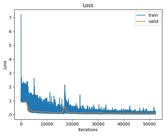
Load the checkpoint trained by us. Do not run this block if you have trained your model in the previous block.

!mkdir -p temp/models/WaterDropSample

simulator = LearnedSimulator()
simulator = simulator.cuda()

!wget -O temp/models/WaterDropSample/checkpoint_100000.pt https://github.com/kks32-courses/sciml/raw/main/lectures/12-gnn/checkpoint_100000.pt

checkpoint = torch.load("temp/models/WaterDropSample/checkpoint_100000.pt")
simulator.load_state_dict(checkpoint["model"])

--2023-11-02 16:18:21--  https://github.com/kks32-courses/sciml/raw/main/lectures/12-gnn/checkpoint_52000.pt
Resolving github.com (github.com)... 192.30.255.112
Connecting to github.com (github.com)|192.30.255.112|:443... connected.
HTTP request sent, awaiting response... 302 Found
Location: https://raw.githubusercontent.com/kks32-courses/sciml/main/lectures/12-gnn/checkpoint_52000.pt [following]
--2023-11-02 16:18:21--  https://raw.githubusercontent.com/kks32-courses/sciml/main/lectures/12-gnn/checkpoint_52000.pt
Resolving raw.githubusercontent.com (raw.githubusercontent.com)... 185.199.108.133, 185.199.109.133, 185.199.110.133, ...
Connecting to raw.githubusercontent.com (raw.githubusercontent.com)|185.199.108.133|:443... connected.
HTTP request sent, awaiting response... 200 OK
Length: 19329754 (18M) [application/octet-stream]
Saving to: ‘temp/models/WaterDropSmall/checkpoint_52000.pt’

temp/models/WaterDr 100%[===================>]  18.43M  --.-KB/s    in 0.1s    

2023-11-02 16:18:23 (172 MB/s) - ‘temp/models/WaterDropSmall/checkpoint_52000.pt’ saved [19329754/19329754]

<All keys matched successfully>

Visualization

Since the video is 1000 frames long, it might take a few minutes to rollout.

rollout_dataset = RolloutDataset(data_path, "valid")
simulator.eval()
rollout_data = rollout_dataset[0]
rollout_out = rollout(simulator, rollout_data, rollout_dataset.metadata, params["noise"])
rollout_out = rollout_out.permute(1, 0, 2)

%matplotlib inline
import matplotlib.pyplot as plt
from matplotlib import animation
from IPython.display import HTML

TYPE_TO_COLOR = {
    3: "black",
    0: "green",
    7: "magenta",
    6: "gold",
    5: "blue",
}


def visualize_prepare(ax, particle_type, position, metadata):
    bounds = metadata["bounds"]
    ax.set_xlim(bounds[0][0], bounds[0][1])
    ax.set_ylim(bounds[1][0], bounds[1][1])
    ax.set_xticks([])
    ax.set_yticks([])
    ax.set_aspect(1.0)
    points = {type_: ax.plot([], [], "o", ms=2, color=color)[0] for type_, color in TYPE_TO_COLOR.items()}
    return ax, position, points


def visualize_pair(particle_type, position_pred, position_gt, metadata):
    fig, axes = plt.subplots(1, 2, figsize=(10, 5))
    plot_info = [
        visualize_prepare(axes[0], particle_type, position_gt, metadata),
        visualize_prepare(axes[1], particle_type, position_pred, metadata),
    ]
    axes[0].set_title("Ground truth")
    axes[1].set_title("Prediction")

    plt.close()

    def update(step_i):
        outputs = []
        for _, position, points in plot_info:
            for type_, line in points.items():
                mask = particle_type == type_
                line.set_data(position[step_i, mask, 0], position[step_i, mask, 1])
            outputs.append(line)
        return outputs

    return animation.FuncAnimation(fig, update, frames=np.arange(0, position_gt.size(0)), interval=10, blit=True)

anim = visualize_pair(rollout_data["particle_type"], rollout_out, rollout_data["position"], rollout_dataset.metadata)
HTML(anim.to_html5_video())